1.6: Inverse Functions

A fashion designer is travelling to Milan for a fashion show. He asks his assistant, Betty, what 75 degrees Fahrenheit is in Celsius, and after a quick search on Google, she finds the formula $C=\dfrac{5}{9} (F-32)$. Using this formula, she calculates $\dfrac{5}{9} (75-32)\approx 24$degrees Celsius. The next day, the designer sends his assistant the week’s weather forecast for Milan, and asks her to convert the temperatures to Fahrenheit.

At first, Betty might consider using the formula she has already found to do the conversions. After all, she knows her algebra, and can easily solve the equation for $F$ after substituting a value for $C$. For example, to convert 26 degrees Celsius, she could write:

$$26 = \dfrac{5}{9}(F - 32)\nonumber$$

$$26 \cdot \dfrac{9}{5} = F - 32\nonumber$$

$$F = 26 \cdot \dfrac{9}{5} + 32 \approx 79\nonumber$$

After considering this option for a moment, she realizes that solving the equation for each of the temperatures would get awfully tedious, and realizes that since evaluation is easier than solving, it would be much more convenient to have a different formula, one which takes the Celsius temperature and outputs the Fahrenheit temperature. This is the idea of an inverse function, where the input becomes the output and the output becomes the input.

Definition: Inverse function

If $f(a)=b$, then a function $g(x)$ is an inverse of $f$ if $g(b)=a$.

The inverse of $f(x)$ is typically notated $f^{-1} (x)$, which is read “$f$ inverse of $x$”, so equivalently, if $f(a)=b$ then $f^{-1} (b)=a$.

Important: The raised -1 used in the notation for inverse functions is simply a notation, and does not designate an exponent or power of -1.

Example $\PageIndex{1}$

If for a particular function, $f(2)=4$, what do we know about the inverse?

Solution

The inverse function reverses which quantity is input and which quantity is output, so if $f(2)=4$, then $f^{-1} (4)=2$.

Alternatively, if you want to re-name the inverse function $g(x)$, then $g(4) = 2$

Exercise $\PageIndex{1}$

Given that $h^{-1} (6)=2$, what do we know about the original function $h(x)$?

Answer

$g(2) = 6$

Notice that original function and the inverse function undo each other. If $f(a)=b$, then $f^{-1} (b)=a$, returning us to the original input. More simply put, if you compose these functions together you get the original input as your answer.

$$f^{-1} (f(a))=a\text{ and }f(f^{-1} (b))=b$$

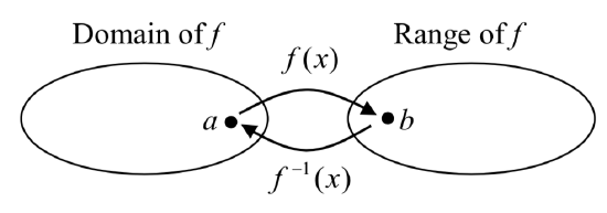
Since the outputs of the function $f$ are the inputs to $f^{-1}$, the range of $f$ is also the domain of $f^{-1}$. Likewise, since the inputs to $f$ are the outputs of $f^{-1}$, the domain of $f$ is the range of $f^{-1}$.

Basically, like how the input and output values switch, the domain & ranges switch as well. But be careful, because sometimes a function doesn’t even have an inverse function, or only has an inverse on a limited domain. For example, the inverse of $f(x)=\sqrt{x}$ is $f^{-1} (x)=x^{2}$, since a square “undoes” a square root, but it is only the inverse of $f(x)$ on the domain $[0, \infty)$, since that is the range of $f(x)=\sqrt{x}$.

Example $\PageIndex{2}$

The function $f(x)=2^{x}$ has domain $(-\infty ,\infty )$ and range $(0,\infty )$, what would we expect the domain and range of $f^{-1}$ to be?

Solution

We would expect $f^{-1}$ to swap the domain and range of $f$, so $f^{-1}$ would have domain $(0,\infty )$ and range $(-\infty ,\infty )$.

Example $\PageIndex{3}$

A function $f(t)$ is given as a table below, showing distance in miles that a car has traveled in $t$ minutes. Find and interpret $f^{-1} (70)$

$t$ (minutes)	30	50	70	90
$f(t)$ (miles)	20	40	60	70

Solution

The inverse function takes an output of $f$ and returns an input for $f$. So in the expression $f^{-1} (70)$, the 70 is an output value of the original function, representing 70 miles. The inverse will return the corresponding input of the original function $f$, 90 minutes, so $f^{-1} (70)=90$. Interpreting this, it means that to drive 70 miles, it took 90 minutes.

Alternatively, recall the definition of the inverse was that if $f(a)=b$ then $f^{-1} (b)=a$. By this definition, if you are given $f^{-1} (70)=a$ then you are looking for a value a so that $f(a)=70$. In this case, we are looking for a $t$ so that $f(t)=70$, which is when $t = 90$.

Exercise $\PageIndex{2}$

Using the table below

$t$ (minutes)	30	50	60	70	90
$f(t)$ (miles)	20	40	50	60	70

Find and interpret the following

a. $f(60)$

b. $f^{-1} (60)$

Answer

a. $f(60) = 50$. In 60 minutes, 50 miles are traveled.

b. $f^{-1}(60) = 70$. To travel 60 miles, it will take 70 minutes.

Example $\PageIndex{4}$

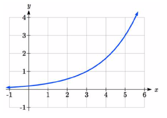
A function $g(x)$ is given as a graph below. Find $g(3)$ and $g^{-1} (3)$

Solution

To evaluate $g(3)$, we find 3 on the horizontal axis and find the corresponding output value on the vertical axis. The point (3, 1) tells us that $g(3)=1$

To evaluate $g^{-1} (3)$, recall that by definition $g^{-1} (3)$ means $g(x) = 3$. By looking for the output value 3 on the vertical axis we find the point (5, 3) on the graph, which means $g(5) = 3$, so by definition $g^{-1} (3) =5$.

Exercise $\PageIndex{3}$

Using the graph in Example 4 above

a. find $g^{-1} (1)$

b. estimate $g^{-1} (4)$

Answer

a. $g^{-1} (1) = 3$

b. $g^{-1} (4) = 5.5$ (this is an approximation - answers may vary slightly)

Example $\PageIndex{5}$

Returning to our designer’s assistant, find a formula for the inverse function that gives Fahrenheit temperature given a Celsius temperature.

Solution

A quick Google search would find the inverse function, but alternatively, Betty might look back at how she solved for the Fahrenheit temperature for a specific Celsius value, and repeat the process in general

$$\begin{array}{l} {C=\dfrac{5}{9} (F-32)} \\ {C\cdot \dfrac{9}{5} =F-32} \\ {F=\dfrac{9}{5} C+32} \end{array}\nonumber$$

By solving in general, we have uncovered the inverse function. If

$$C=h(F)=\dfrac{5}{9} (F-32)\nonumber$$

Then

$$F=h^{-1} (C)=\dfrac{9}{5} C+32\nonumber$$

In this case, we introduced a function h to represent the conversion since the input and output variables are descriptive, and writing $C^{-1}$could get confusing.

It is important to note that not all functions will have an inverse function. Since the inverse $f^{-1} (x)$ takes an output of $f$ and returns an input of $f$, in order for $f^{-1}$ to itself be a function, then each output of $f$ (input to $f^{-1}$) must correspond to exactly one input of $f$ (output of $f^{-1}$) in order for $f^{-1}$ to be a function. You might recall that this is the definition of a one-to-one function.

Definition: Properties of inverses

In order for a function to have an inverse, it must be a one-to-one function.

In some cases, it is desirable to have an inverse for a function even though the function is not one-to-one. In those cases, we can often limit the domain of the original function to an interval on which the function is one-to-one, then find an inverse only on that interval.

If you have not already done so, go back to the toolkit functions that were not one-to-one and limit or restrict the domain of the original function so that it is one-to-one. If you are not sure how to do this, proceed to Example 6.

Example $\PageIndex{6}$

The quadratic function $h(x)=x^{2}$ is not one-to-one. Find a domain on which this function is one-to-one, and find the inverse on that domain.

Solution

We can limit the domain to $[0,\infty )$to restrict the graph to a portion that is one-to-one, and find an inverse on this limited domain.

You may have already guessed that since we undo a square with a square root, the inverse of $h(x)=x^{2}$ on this domain is $h^{-1} (x)=\sqrt{x}$.

You can also solve for the inverse function algebraically. If $h(x)=x^{2}$, we can introduce the variable $y$ to represent the output values, allowing us to write $y=x^{2}$. To find the inverse we solve for the input variable

To solve for $x$ we take the square root of each side. $\sqrt{y} =\sqrt{x^{2} }$ and get $\sqrt{y} =|x|$, so $x=\pm \sqrt{y}$. We have restricted $x$ to being non-negative, so we’ll use the positive square root, $x=\sqrt{y}$ or $h^{-1} (y)=\sqrt{y}$. In cases like this where the variables are not descriptive, it is common to see the inverse function rewritten with the variable $x$: $h^{-1} (x)=\sqrt{x}$. Rewriting the inverse using the variable $x$ is often required for graphing inverse functions using calculators or computers.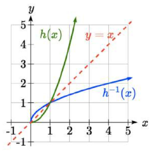

Note that the domain and range of the square root function do correspond with the range and domain of the quadratic function on the limited domain. In fact, if we graph $h(x)$ on the restricted domain and $h^{-1} (x)$ on the same axes, we can notice symmetry: the graph of $h^{-1} (x)$ is the graph of h(x) reflected over the line $y = x$.

Example $\PageIndex{7}$

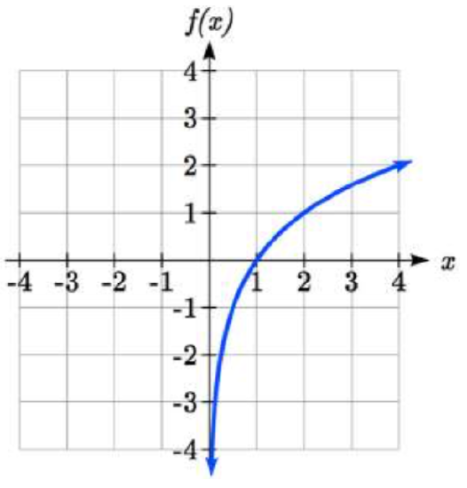
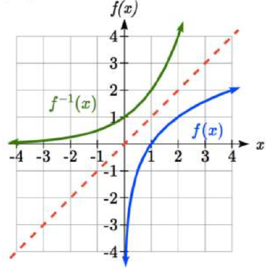
Given the graph of $f(x)$ shown, sketch a graph of $f^{-1} (x)$.

Solution

This is a one-to-one function, so we will be able to sketch an inverse. Note that the graph shown has an apparent domain of $(0, \infty)$ and range of $(-\infty, \infty)$, so the inverse will have a domain of $(-\infty, \infty)$ and range of $(0, \infty)$.

Reflecting this graph of the line $y = x$, the point (1, 0) reflects to (0, 1), and the point (4, 2) reflects to (2, 4). Sketching the inverse on the same axes as the original graph:

Important Topics of this Section

Definition of an inverse function

Composition of inverse functions yield the original input value

Not every function has an inverse function

To have an inverse a function must be one-to-one

Restricting the domain of functions that are not one-to-one.