3.6: Dividing Fractions

You are probably familiar with the computational rule on how to divide fractions: to divide by a fraction, multiply by its reciprocal, which is also known as the invert and multiply rule. In this section, we provide context to understand why this rule works. Does it really make sense? Can you explain why it makes sense?

Definition: Invert an Multiply Rule

\(\dfrac{a}{b}\div\dfrac{c}{d}=\dfrac{a}{b}\times\dfrac{d}{c}=\dfrac{ad}{bc}\)

We are going to build up to the invert and multiply rule, but along the way, we’ll find some more meaningful ways to understand division of fractions. So please play along: pretend that you don’t already know the invert and multiply rule, and solve the problems in this chapter with other methods.

Equal-Sized Groups Approach

The division: \(18 \div 3\) means: How many groups of 3 can I find in 18?

We start with 18 dots, and we make groups of 3 dots. We ask: how many groups can we make?

Figure \(\PageIndex{1}\): 18 dots, split into groups of 3 dots. Since there are 6 groups, we have \(18\div 3 = 6\).

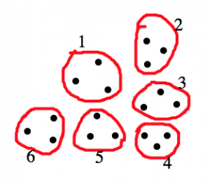
This same idea applies when we divide fractions. Consider the following example. For example, \(6 \div \dfrac{2}{3}\) means: How many groups of \(\dfrac{2}{3}\) can I find in 6?

Example \(\PageIndex{1}\)

How many groups of size \(\frac{2}{3}\) can I find in 6?

Solution

Let’s draw a picture of 6 pies, and see how many groups of \(\frac{2}{3}\) we can find:

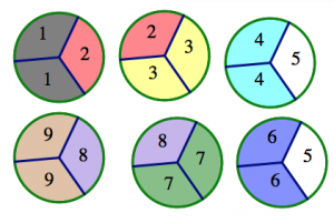
We found nine equal groups of size \(\frac{2}{3}\), so we conclude that \[6 \div \frac{2}{3} = 9 \ldotp \nonumber \]

Unfortunately, it’s not always quite so straightforward to find the equal groups. For example, \(\frac{3}{4} \div \frac{1}{3}\) asks the question: How many groups of \(\frac{1}{3}\) can I find in \(\frac{3}{4}\)?

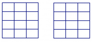
Here’s a method that lets you compute exactly. We’ll use rectangular pies and divide them into rows and columns based on the denominators of the numbers we’re dividing.

Example \(\PageIndex{1}\)

Represent the division: \(\dfrac{3}{4}\div\dfrac{1}{3}\)

Solution

Start by drawing two identical rectangles, each with 4 rows (from the denominator of \(\dfrac{3}{4}\) and 3 columns (from the denominator of \(\dfrac{1}{3}\)).

Shade \(\dfrac{3}{4}\) of the first rectangle (this is exactly three rows), and shade \(\dfrac{1}{3}\) of the second rectangle (so that’s one column).

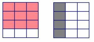
Now ask: how many copies of \(\dfrac{1}{3}\) can I find in \(\dfrac{3}{4}\)? Well, \(\dfrac{1}{3}\) is equal to four of the smaller squares. So we find groups equal to that:

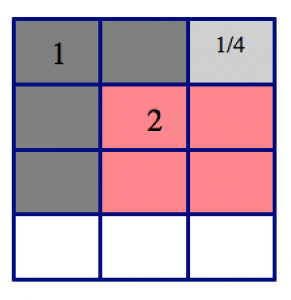
In the picture of \(\dfrac{3}{4}\), we can find:

• two groups of four squares (two groups of \(\dfrac{1}{3}\)), and
• one square left over, which is \(\dfrac{1}{4}\) of the group we’re looking for.

We conclude: \[\dfrac{3}{4} \div \dfrac{1}{3} = 2 \dfrac{1}{4} \ldotp \nonumber \]

Think / Pair / Share

Discussion:

Determine the quotient by using the equal-sized groups approach: \(\dfrac{3}{4} \div \dfrac{1}{2}\)

Common Denominator Method

Discussion:

Solve each of the following fraction division problems using the equal-sized groups approach:

• \(\dfrac{6}{4} \div \dfrac{3}{4}\)
• \(\dfrac{6}{10} \div \dfrac{3}{10}\)
• \(\dfrac{8}{9} \div \dfrac{4}{9}\)
• \(\dfrac{6}{33} \div \dfrac{2}{33}\)
• \(\dfrac{5}{4} \div \dfrac{2}{4}\)
• \(\dfrac{5}{2} \div \dfrac{2}{2}\)
• \(\dfrac{5}{10} \div \dfrac{2}{10}\)

What do you notice?

When dividing fractions of the same denominator, the result is the ratio of both numerators. We leverage this as a tool for creating our first method for dividing two fractions.

Definition: Common Denominator Method

If two fractions have the same denominator, then when you divide them, you can just divide the numerators. In symbols, \[\dfrac{a}{d} \div \dfrac{b}{d} = \dfrac{a}{b} \ldotp \nonumber \]

Discussion:

• Use the common denominator method to find these quotients:
• \(\dfrac{1}{3} \div \dfrac{2}{3}\)
• What if the fractions do not have a common denominator? Is the method useless, or can you find a way to make it work? Can you solve these problems?\(\dfrac{3}{5} \div \dfrac{3}{4}\)

Missing Factor Method

We know we can always turn a division problem into a missing-factor multiplication problem. This is a tool for computing fraction division.

Discussion:

Rewrite the problems below as a missing factor multiplication question. Then find the quotient using what you know about multiplying fractions.

• \(\dfrac{9}{10} \div \dfrac{3}{5}\)
• \(\dfrac{7}{8} \div \dfrac{1}{4}\)

Unfortunately, the missing factor method doesn’t always work out so nicely. For example,

\[\dfrac{3}{4} \div \dfrac{1}{3} = \_\_ \nonumber \]

can be rewritten as

\[\dfrac{1}{3} \cdot \_\_ = \dfrac{3}{4} \ldotp \nonumber \]

You want to ask:

• For the numerator: \(1 \cdot \_\_ = 3\). We can fill in the blank with a 3.
• For the denominator: \(3 \cdot \_\_ = 4\). We can fill in the blank with \(\frac{4}{3}\). (Why does that work?)

So we have: \(\dfrac{1}{3} \cdot \dfrac{3}{\frac{4}{3}} = \dfrac{3}{4} \ldotp \nonumber \)

In the context of the Pie per Child Model, \(\dfrac{3}{\frac{4}{3}}\) means that each \(\dfrac{4}{3}\) of a kid gets 3 pies. So how much does an individual kid get? You could draw a picture to help you figure it out. But we can also use the key fraction rule to help us out.

\[\frac{3}{\frac{4}{3}} = \frac{3 \cdot 3}{3 \cdot \frac{4}{3}} = \frac{9}{4} \ldotp \nonumber \]

The Simplification Method

To understand the invert and multiply rule, let's consider the following problem: \(7 \frac{2}{3}\) pies are shared equally by \(5 \frac{1}{4}\) children. How much pie does each child get?

Technically, we could just write down the answer as \(\dfrac{7 \frac{2}{3}}{5 \frac{1}{4}}\) and be done! The answer is equivalent to this fraction, so why not?

Is there a way to make this look friendlier? Well, if we change those mixed numbers to improper fractions, it helps a little:

\(\dfrac{7 \frac{2}{3}}{5 \frac{1}{4}} = \dfrac{\frac{23}{3}}{\frac{21}{4}} \nonumber \)

That’s a bit better, but it’s still not clear how much pie each kid gets. Let’s use the key fraction rule to make the fraction even friendlier. Let’s multiply the numerator and denominator each by 3. Remember, multiplying by 3 means we’re multiplying the fraction by \(\dfrac{3}{3}\), which is just a special form of 1, so we don’t change its value.

\[\dfrac{3 \cdot \frac{23}{3}}{3 \cdot \frac{21}{4}} = \dfrac{23}{\frac{63}{4}} \ldotp \nonumber \]

Now multiply numerator and denominator each by 4, which will not change the value as we would be multiplying by \(dfrac{4}{4}\).

\[\dfrac{4 \cdot 23}{4 \cdot \frac{63}{4}} = \dfrac{92}{63} \ldotp \nonumber \]

We now see that the answer is \(\dfrac{92}{63}\). That means that sharing \(7 \dfrac{2}{3}\) pies among \(5 \dfrac{1}{4}\) children is the same as sharing 92 pies among 63 children. Notice that, in both situations, the individual child gets exactly the same amount of pie.

Thinking about this process leads to an equivalent way of justifying the invert and multiply rule. Without a context, we can consider the following problem.

Example \(\PageIndex{1}\)

Use the simplification method illustrated above to solve the following:\(\dfrac{3}{5}}\div{\dfrac{2}{3}\)

Solution

First, rewrite the problem in the following way: \[\dfrac{\frac{3}{5}}{\frac{2}{3}} \ldotp \nonumber \]

Multiplying the numerator and denominator each by 5 (why did we choose 5?) gives

\[\dfrac{\frac{3}{5}}{\frac{2}{3}} = \dfrac{5 \cdot \frac{3}{5}}{5 \cdot \frac{2}{3}} = \dfrac{3}{\frac{10}{3}} \ldotp \nonumber \]

Now multiply the numerator and denominator each by 3 (why did we choose 3?):

\[\dfrac{3 \cdot 3}{3 \cdot \frac{10}{3}} = \dfrac{9}{10} \ldotp \nonumber \]

Perhaps without realizing it, we have rediscovered the invert multiply method for dividing fractions.

Invert and Multiply

We can think about the invert and multiply method as a shortcut of the simplification method, this is because the process justifies the following result:

\[\dfrac{a}{b}\div\dfrac{c}{d}=\dfrac{a}{b}\times\dfrac{d}{c}=\dfrac{ad}{bc}\]

Example \(\PageIndex{1}\)

Consider \(\frac{5}{9} \div \frac{8}{11}\):

Solution

\[\frac{5}{9} \div \frac{8}{11} = \frac{\frac{5}{9}}{\frac{8}{11}} \ldotp \nonumber \]

Let’s multiply numerator and denominator each by 9 and by 11 at the same time. (Why not?)

\[\frac{\frac{5}{9}}{\frac{8}{11}} = \frac{(\frac{5}{9}) \cdot 9 \cdot 11}{(\frac{8}{11}) \cdot 9 \cdot 11} = \frac{5 \cdot 11}{8 \cdot 9} \ldotp \nonumber \]

(Do you see what happened here?)

So we have

\[\frac{\frac{5}{9}}{\frac{8}{11}} = \frac{5 \cdot 11}{8 \cdot 9} = \frac{55}{72} \ldotp \nonumber \]

Discussion:

Consider the problem \(\frac{5}{12} \div \frac{7}{11}\). Janine wrote:

\[\frac{\frac{5}{12}}{\frac{7}{11}} = \frac{\frac{5}{12} \cdot 12 \cdot 11}{\frac{7}{11} \cdot 12 \cdot 11} = \frac{5 \cdot 11}{7 \cdot 12} = \frac{5}{12} \cdot \frac{11}{7} \ldotp \nonumber \]

She stopped before completing her final step and exclaimed: “Dividing one fraction by another is the same as multiplying the first fraction with the second fraction upside down!”

Check each step of Janine’s work here and ensure it is correct. Then answer these questions:

• Do you understand what Janine is saying? Explain it very clearly.
• Work out \(\frac{\frac{3}{7}}{\frac{4}{13}}\) using the simplification method. Is the answer the same as \(\frac{3}{7} \cdot \frac{13}{4}\)?
• Work out \(\frac{\frac{2}{5}}{\frac{3}{10}}\) using the simplification method. Is the answer the same as \(\frac{2}{5} \cdot \frac{10}{3}\)?
• Work out \(\frac{\frac{a}{b}}{\frac{c}{d}}\) using the simplification method. Is the answer the same as \(\frac{a}{b} \cdot \frac{d}{c}\)?
• Is Janine right? Is dividing two fractions always the same as multiplying the two fractions with the second one turned upside down? What do you think? Do not just think about examples. This is a question of whether something is always true.

Summary

We now have several methods for solving problems that require dividing fractions:

Dividing fractions:

• Equal-sized groups approach: Draw a picture using the rectangle method, and use that to solve the division problem.
• Common Denominator Method: Find a common denominator and divide the numerators.
• Missing Factor Method: Rewrite the division as a missing factor multiplication problem, and solve that problem.
• Simplification Method: Simplify an ugly fraction.
• Invert and Multiply Method: Invert the second fraction (the dividend) and then multiply.