3.5: Multiplying Fractions

Area Model

We can represent multiplication of numbers by using area models. For example, the product \(23 \times 37\) is the area (number of 1 × 1 squares) of a 23-by-37 rectangle:

Figure \(\PageIndex{1}\): The product of \(23 \times 37\) represented in an area model.

So the product of two fractions, say, \(\dfrac{4}{7} \times \dfrac{2}{3}\) should also correspond to an area problem. The figures below illustrate the process of connecting the multiplication \(\dfrac{4}{7} \times \dfrac{2}{3}\) with an area model.

Figure \(\PageIndex{1}\): Step 1: Draw a segment of some length; we call this a 1 unit.

Figure \(\PageIndex{1}\): Step 2: Draw a square with one unit on each side.

Figure \(\PageIndex{1}\): Step 3: Mark the square. The segment on the top represents a segment split into 3 parts, each of size \(\frac{1}{3}\) and the segment on the side represents 7 pieces of size \(\frac{1}{7}\).

Figure \(\PageIndex{1}\): Step 4: Draw rectangles with one side that measures \(\frac{1}{3}\) and another side that measures \(\frac{1}{7}\).

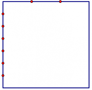
The area of the square is \(1 \times 1 = 1\) square unit. The marks in the square divide the whole square into small, equal-sized rectangles. Resulting in 21 smaller rectangles, each representing the multiplication \(\dfrac{1}{7} \times \dfrac{1}{3}\).

We can now mark off four sevenths on one side and two-thirds on the other side. This supports the appropriate shading for the rectangles to solve the multiplication \(\dfrac{4}{7} \times \dfrac{2}{3}\)

Figure \(\PageIndex{1}\): \(\dfrac{4}{7} \times \dfrac{2}{3}\)

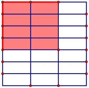
The result of the multiplication should be the area of the rectangle with \(\frac{4}{7}\) on one side and \(\frac{2}{3}\) on the other. What is that area?

Remember, the whole square was one unit. That one-unit square is divided into 21 equal-sized pieces, and the shaded area contains eight of those rectangles. Since the shaded area is the answer to our multiplication problem, we conclude that

\[\frac{4}{7} \times \frac{2}{3} = \frac{8}{21} \ldotp \nonumber \]

Discuss:

1. The area problem \(\dfrac{4}{7} \times \dfrac{2}{3}\) yielded a diagram with a total of 21 small rectangles. Explain why 21 appears as the total number of equal-sized rectangles.
2. The area problem \(\dfrac{4}{7} \times \dfrac{2}{3}\) yielded a diagram with 8 small shaded rectangles. Explain why 8 appears as the number of shaded rectangles.
3. How can you extend the area model for fractions greater than 1? Try to draw a picture for: \(\dfrac{3}{4} \cdot \dfrac{3}{2}\).

Explaining the Multiplication Rule

Definition: Multiplication of Fractions

\[\frac{a}{b} \cdot \frac{c}{d} = \frac{a \cdot c}{b \cdot d} \ldotp \nonumber \]

Of course, you may then choose to simplify the final answer, but the answer is always equivalent to this one. Why? The area model can help us explain what is going on.

First, let us clearly write out how the area model says to multiply \(\dfrac{a}{b} \cdot \dfrac{c}{d}\). We want to build a rectangle where one side has length \(\dfrac{a}{b}\) and the other side has length \(\dfrac{c}{d}\). We start with a square, one unit on each side.

• Divide the top segment into \(b\) equal-sized pieces. Shade \(a\) of those pieces. This will be the side of the rectangle with length \(\dfrac{a}{b}\).
• Divide the left segment into \(d\) equal-sized pieces. Shade \(c\) of those pieces. This will be the side of the rectangle with length \(\dfrac{c}{d}\).
• Divide the whole rectangle according to the tick marks on the sides, making equal-sized rectangles.
• Shade the rectangle bounded by the shaded segments.

If the answer is \(\dfrac{a \cdot c}{b \cdot d}\), that means there are \(b \cdot d\) total equal-sized pieces in the square, and \(a \cdot c\) of them are shaded. We can see from the model why this is the case:

• The top segment was divided into \(b\) equal-sized pieces. So there are \(b\) columns in the rectangle.
• The side segment was divided into \(d\) equal-sized pieces. So there are \(d\) rows in the rectangle.
• A rectangle with \(b\) columns and \(d\) rows has \(b \cdot d\) pieces, which is the area model for whole-number multiplication!

Discussion:

Consider the Definition of the Multiplication of Fraction: \[\dfrac{a}{b} \cdot \dfrac{c}{d} = \dfrac{a \cdot c}{b \cdot d} \ldotp \nonumber \]

Write a clear explanation for why \(a \cdot c\) of the small rectangles will be shaded.

Multiplying Fractions by Whole Numbers

To multiply \(2 \cdot \dfrac{3}{7}\), you may think of “2” as \(\dfrac{2}{1}\), the whole number with a denominator of one, and compute this way \[2 \cdot \dfrac{3}{7} = \dfrac{2}{1} \cdot \dfrac{3}{7} = \dfrac{2 \cdot 3}{1 \cdot 7} = \dfrac{6}{7} \ldotp \nonumber \]

We can also think in terms of our original Pies Per Child Model to answer questions like this. In this case, we know that \(\dfrac{3}{7}\) means the amount of pie each child gets when 7 children evenly share 3 pies.

If we compute \(2 \cdot \dfrac{3}{7}\) that means we double the amount of pie each kid gets. We can do this by doubling the number of pies. So the answer is the same as \(\dfrac{6}{7}\): the amount of pie each child gets when 7 children evenly share 6 pies.

Finally, we can think in terms of the whole as a unit. The fraction \(\dfrac{3}{7}\) means that I have 7 equal pieces (of something), and I take 3 of them. So \(2 \cdot \dfrac{3}{7}\) means do that twice. If I take 3 pieces and then 3 pieces again, I get a total of 6 pieces. There are still 7 equal pieces in the whole, so the answer is \(\dfrac{6}{7}\).

Discussion:

1. Use all three methods to explain how to find the product: \(3 \cdot \dfrac{2}{5}\)
2. Compare these different ways of thinking about fraction multiplication. Are any of them more natural to you? Does one make more sense than the others? Do the particular numbers in the problem affect your answer? Compare your thoughts with what other's think in your class. Do they agree?