
4.3: Measures of Central Tendency
- Page ID
- 92988

\( \newcommand{\vecs}[1]{\overset { \scriptstyle \rightharpoonup} {\mathbf{#1}} } \)
\( \newcommand{\vecd}[1]{\overset{-\!-\!\rightharpoonup}{\vphantom{a}\smash {#1}}} \)
\( \newcommand{\dsum}{\displaystyle\sum\limits} \)
\( \newcommand{\dint}{\displaystyle\int\limits} \)
\( \newcommand{\dlim}{\displaystyle\lim\limits} \)
\( \newcommand{\id}{\mathrm{id}}\) \( \newcommand{\Span}{\mathrm{span}}\)
( \newcommand{\kernel}{\mathrm{null}\,}\) \( \newcommand{\range}{\mathrm{range}\,}\)
\( \newcommand{\RealPart}{\mathrm{Re}}\) \( \newcommand{\ImaginaryPart}{\mathrm{Im}}\)
\( \newcommand{\Argument}{\mathrm{Arg}}\) \( \newcommand{\norm}[1]{\| #1 \|}\)
\( \newcommand{\inner}[2]{\langle #1, #2 \rangle}\)
\( \newcommand{\Span}{\mathrm{span}}\)
\( \newcommand{\id}{\mathrm{id}}\)
\( \newcommand{\Span}{\mathrm{span}}\)
\( \newcommand{\kernel}{\mathrm{null}\,}\)
\( \newcommand{\range}{\mathrm{range}\,}\)
\( \newcommand{\RealPart}{\mathrm{Re}}\)
\( \newcommand{\ImaginaryPart}{\mathrm{Im}}\)
\( \newcommand{\Argument}{\mathrm{Arg}}\)
\( \newcommand{\norm}[1]{\| #1 \|}\)
\( \newcommand{\inner}[2]{\langle #1, #2 \rangle}\)
\( \newcommand{\Span}{\mathrm{span}}\) \( \newcommand{\AA}{\unicode[.8,0]{x212B}}\)
\( \newcommand{\vectorA}[1]{\vec{#1}} % arrow\)
\( \newcommand{\vectorAt}[1]{\vec{\text{#1}}} % arrow\)
\( \newcommand{\vectorB}[1]{\overset { \scriptstyle \rightharpoonup} {\mathbf{#1}} } \)
\( \newcommand{\vectorC}[1]{\textbf{#1}} \)
\( \newcommand{\vectorD}[1]{\overrightarrow{#1}} \)
\( \newcommand{\vectorDt}[1]{\overrightarrow{\text{#1}}} \)
\( \newcommand{\vectE}[1]{\overset{-\!-\!\rightharpoonup}{\vphantom{a}\smash{\mathbf {#1}}}} \)
\( \newcommand{\vecs}[1]{\overset { \scriptstyle \rightharpoonup} {\mathbf{#1}} } \)
\(\newcommand{\longvect}{\overrightarrow}\)
\( \newcommand{\vecd}[1]{\overset{-\!-\!\rightharpoonup}{\vphantom{a}\smash {#1}}} \)
\(\newcommand{\avec}{\mathbf a}\) \(\newcommand{\bvec}{\mathbf b}\) \(\newcommand{\cvec}{\mathbf c}\) \(\newcommand{\dvec}{\mathbf d}\) \(\newcommand{\dtil}{\widetilde{\mathbf d}}\) \(\newcommand{\evec}{\mathbf e}\) \(\newcommand{\fvec}{\mathbf f}\) \(\newcommand{\nvec}{\mathbf n}\) \(\newcommand{\pvec}{\mathbf p}\) \(\newcommand{\qvec}{\mathbf q}\) \(\newcommand{\svec}{\mathbf s}\) \(\newcommand{\tvec}{\mathbf t}\) \(\newcommand{\uvec}{\mathbf u}\) \(\newcommand{\vvec}{\mathbf v}\) \(\newcommand{\wvec}{\mathbf w}\) \(\newcommand{\xvec}{\mathbf x}\) \(\newcommand{\yvec}{\mathbf y}\) \(\newcommand{\zvec}{\mathbf z}\) \(\newcommand{\rvec}{\mathbf r}\) \(\newcommand{\mvec}{\mathbf m}\) \(\newcommand{\zerovec}{\mathbf 0}\) \(\newcommand{\onevec}{\mathbf 1}\) \(\newcommand{\real}{\mathbb R}\) \(\newcommand{\twovec}[2]{\left[\begin{array}{r}#1 \\ #2 \end{array}\right]}\) \(\newcommand{\ctwovec}[2]{\left[\begin{array}{c}#1 \\ #2 \end{array}\right]}\) \(\newcommand{\threevec}[3]{\left[\begin{array}{r}#1 \\ #2 \\ #3 \end{array}\right]}\) \(\newcommand{\cthreevec}[3]{\left[\begin{array}{c}#1 \\ #2 \\ #3 \end{array}\right]}\) \(\newcommand{\fourvec}[4]{\left[\begin{array}{r}#1 \\ #2 \\ #3 \\ #4 \end{array}\right]}\) \(\newcommand{\cfourvec}[4]{\left[\begin{array}{c}#1 \\ #2 \\ #3 \\ #4 \end{array}\right]}\) \(\newcommand{\fivevec}[5]{\left[\begin{array}{r}#1 \\ #2 \\ #3 \\ #4 \\ #5 \\ \end{array}\right]}\) \(\newcommand{\cfivevec}[5]{\left[\begin{array}{c}#1 \\ #2 \\ #3 \\ #4 \\ #5 \\ \end{array}\right]}\) \(\newcommand{\mattwo}[4]{\left[\begin{array}{rr}#1 \amp #2 \\ #3 \amp #4 \\ \end{array}\right]}\) \(\newcommand{\laspan}[1]{\text{Span}\{#1\}}\) \(\newcommand{\bcal}{\cal B}\) \(\newcommand{\ccal}{\cal C}\) \(\newcommand{\scal}{\cal S}\) \(\newcommand{\wcal}{\cal W}\) \(\newcommand{\ecal}{\cal E}\) \(\newcommand{\coords}[2]{\left\{#1\right\}_{#2}}\) \(\newcommand{\gray}[1]{\color{gray}{#1}}\) \(\newcommand{\lgray}[1]{\color{lightgray}{#1}}\) \(\newcommand{\rank}{\operatorname{rank}}\) \(\newcommand{\row}{\text{Row}}\) \(\newcommand{\col}{\text{Col}}\) \(\renewcommand{\row}{\text{Row}}\) \(\newcommand{\nul}{\text{Nul}}\) \(\newcommand{\var}{\text{Var}}\) \(\newcommand{\corr}{\text{corr}}\) \(\newcommand{\len}[1]{\left|#1\right|}\) \(\newcommand{\bbar}{\overline{\bvec}}\) \(\newcommand{\bhat}{\widehat{\bvec}}\) \(\newcommand{\bperp}{\bvec^\perp}\) \(\newcommand{\xhat}{\widehat{\xvec}}\) \(\newcommand{\vhat}{\widehat{\vvec}}\) \(\newcommand{\uhat}{\widehat{\uvec}}\) \(\newcommand{\what}{\widehat{\wvec}}\) \(\newcommand{\Sighat}{\widehat{\Sigma}}\) \(\newcommand{\lt}{<}\) \(\newcommand{\gt}{>}\) \(\newcommand{\amp}{&}\) \(\definecolor{fillinmathshade}{gray}{0.9}\)In addition to graphical and verbal descriptions of data, we can use numbers to summarize quantitative data distributions. We want to know what a typical, average, or representative value for a set of data is (the center of the data), and how spread out the values are in the data set. In this section we explore measures of central tendency, and in the next section we will explore measures of spread.
Mean
We need to be careful with using the word "average" as it means different things to different people in different contexts. One of the most common uses of the word "average" is what mathematicians and statisticians call the arithmetic mean, or just plain old mean for short. The mean is what most people think of when they use the word "average," but we should try to use statistical terms to be precise.
The mean of a set of data is found as the sum of the data values divided by the number of values.
Symbolically, the formula for the sample mean is
\(\overline{x} = \dfrac{\sum x_i}{n}= \dfrac{x_1 + x_2 + x_3 + x_4 + ... + x_n}{n}\)
where each \(x_i\) is the \(i^\text{th}\) data value and \(n\) is the sample size. \(\sum x_i\) is a short way to write a bunch of \(x\)'s added together.
Statisticians use the symbol \(\overline{x}\) to represent the mean while \(x\) is the symbol for a single measurement. We say \(\overline{x}\) as “x bar.”
Marci’s exam scores for her last math class were 79, 86, 82, and 94. What is the mean of Marci's exam scores?
\(\dfrac{79+86+82+94}{4}=85.25\)
Typically, we round means to one more decimal place than the original data had. In this case, we would round 85.25 to 85.3.
The number of touchdown (TD) passes thrown by each of the 31 teams in the National Football League in the 2000 season are shown below. Find the mean number of TD passes.
37 33 33 32 29 28 28 23 22 22 22 21 21 21 20
20 19 19 18 18 18 18 16 15 14 14 14 12 12 9 6
Solution
Adding these values, we get 634 total TDs. Dividing by the number of data values, 31, we get \(\frac{634}{31} \approx 20.4516\). It would be appropriate to round this to 20.5 TDs.
It would be most correct for us to report that “The mean number of touchdown passes thrown in the NFL in the 2000 season was 20.5 passes,” but it is not uncommon to see the more casual word “average” used in place of “mean."
The price of a jar of peanut butter at 5 stores was $3.29, $3.59, $3.79, $3.75, and $3.99. Find the mean price.
- Answer
-
$3.68.
We can also find the mean when data has been organized into a frequency table.
A sample of 100 families in a particular neighborhood are asked their annual household income, to the nearest 5 thousand dollars. The results are summarized in a frequency table below. What is the mean annual household income for this neighborhood?
\(\begin{array}{|c|c|}
\hline \textbf { Income (thousands of dollars) } & \textbf { Frequency } \\
\hline 15 & 6 \\
\hline 20 & 8 \\
\hline 25 & 11 \\
\hline 30 & 17 \\
\hline 35 & 19 \\
\hline 40 & 20 \\
\hline 45 & 12 \\
\hline 50 & 7 \\
\hline
\end{array}\)
Solution
Calculating the mean by hand could get tricky if we try to actually add 100 values. We want to add all 100 values and divide by 100 such as
\(\overline{x} = \dfrac{15 + \cdots + 15 + 20 + \cdots+20 + 25 + \cdots + 25 + \cdots + 50+50}{100} \)
We could calculate this more easily by noticing that adding 15 to itself six times is the same as \(15 \cdot 6=90\). Using this shortcut, we get
\(\overline{x} = \dfrac{15 \cdot 6+20 \cdot 8+25 \cdot 11+30 \cdot 17+35 \cdot 19+40 \cdot 20+45 \cdot 12+50 \cdot 7}{100}=\dfrac{3390}{100}=33.9\)
The mean household income of our sample is 33.9 thousand dollars ($33,900).
Continuing from the previous example, suppose a new family with a household income of 5 million dollars moves into the neighborhood. (This is 5,000 thousand dollars). Including this in the sample, the mean is now
Solution
\(\overline{x} = \dfrac{15 \cdot 6+20 \cdot 8+25 \cdot 11+30 \cdot 17+35 \cdot 19+40 \cdot 20+45 \cdot 12+50 \cdot 7+5000 \cdot 1}{101}=\dfrac{8390}{101} \approx 83.069\)
While 83.1 thousand dollars ($83,100) is the correct mean household income, it no longer represents a “typical” value.
Imagine the data values on a see-saw or balance scale. The mean is the value that keeps the data in balance, like in the picture below.

In the graph of the household income data, the $5 million data value is so far out to the right that the mean has to adjust up to keep things in balance.

For this reason, when working with data sets that have outliers – values far outside the primary grouping – it is common to use a different measure of center -- the median.
Median
Most of us are familiar with the median of a roadway. It is usually an area of grass or concrete that separates two halves of the roadway. The median is defined similarly in statistics.
The median is the value found in the middle of an ordered data set.
There is no symbol or formula for median. To find the median, order (or rank) the data values from smallest to largest and then count from both ends inward towards the center one data value at a time until reaching the middle:
- If there are an odd number of data values, then there is one middle data value and that is the median.
- If there are an even number of data values, then there are two middle data values. The median is the mean of those two data values.
Find the median of these quiz scores: 5 10 8 6 4 8 2 5 7 7 6
Solution
We must start by listing the data in order: 2 4 5 5 6 6 7 7 8 8 10
It is helpful to mark or cross off the numbers in the original data set as you list them to make sure you don’t miss any. Also, be sure to count the number of data values in the ordered list to make sure it matches the number of data values in the original list.
In this example there are \(n=11\) quiz scores. When the distribution contains an odd number of data values, there will be a single value in the middle and that value is the median. For small data sets, we can “walk” one value at a time from the ends of the ordered list towards the center to find the median
\[\underbrace{\text{2 4 5 5 6 }}_{\text{lower half}} \: \: \: \underbrace{\text{ 6 }}_{\text{median}} \: \: \: \underbrace{\text{ 7 7 8 8 10}}_{\text{upper half}} \nonumber\]
The median test score is 6 points.
Suppose another quiz score needs to be included in the set of quiz scores in the previous example. Someone in the class got a perfect score of 20 points on this very difficult quiz.
Solution
The ordered list of data is now: 2 4 5 5 6 6 7 7 8 8 10 20
There are now \(n=12\) quiz scores in our sample. When the distribution contains an even number of data values, there will be a pair of values in the middle rather than a single value. We find the mean of those middle two values.
\[\underbrace{\text{2 4 5 5 6 }}_{\text{lower half}} \: \: \: \underbrace{\text{ 6 7 }}_{\text{middle pair}} \: \: \: \underbrace{\text{ 7 8 8 10 20}}_{\text{upper half}} \nonumber\]
The median test score is \(\dfrac{6 +7}{2}=6.5\) points.
It is important to notice that despite adding an outlier quiz score to the data set, the median is largely unaffected. The median quiz score for the new distribution is 6.5 points when it was 6 points before.
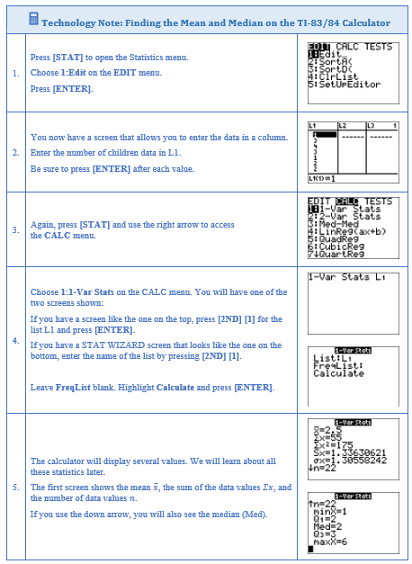
The students in a math class were asked to report the number of children that live in their house (including brothers and sisters temporarily away at college). The data are recorded below. Find the mean and median for these data.
1 3 4 3 1 2 2 2 1 2 2 3 4 5 1 2 3 2 1 2 3 6
Solution
To find the mean, first determine that the sum of all data values is \(\sum x = 55\). Then, divide the sum by the number of data values in the list, \(n=22\). The mean is \(\overline{x} = \frac{55}{22} = 2.5\) children.
To find the median, begin by ordering the data: 1 1 1 1 1 2 2 2 2 2 2 2 2 3 3 3 3 3 4 4 5 6
Because there is an even number of data values (\(n=22\)), the median will be between the two middle values located at position #11 and position #12. The median is \(\frac{2+2}{2} = 2\) children.
For larger data sets, technology will be useful. The procedure for finding the mean and median using a TI calculator is shown.
The Mean vs. the Median
Both the mean and the median are important and widely used measures of center for quantitative data. Is one better to use than the other? It depends -- as the following example shows.
Suppose you got an 85 and a 93 on your first two quizzes, but then you had a really bad day and got a 14 on your next quiz!
- The mean of your three grades is \(\dfrac{85+93+14}{3}=\dfrac{192}{3}=\bf{64}\)
- The median of your three grades is 85 because 85 is in the middle once the data are ordered: 14 85 93.
Which result do you think gives a more accurate picture of your performance?
Solution
The median does not change if the lowest grade is an 84 or if the lowest grade is a 14. However, when you add the three numbers to find the mean, the sum will be much smaller if the lowest grade is a 14. You would probably argue that the median is more representative of your performance because you had done well except for one bad day.
The mean and the median are so different in this example because there is one grade that is extremely different from the rest of the data. In statistics, we call such an extreme value an outlier. The mean is affected by the presence of an outlier; however, the median usually is not affected as much or even at all. A statistic that is not significantly affected by outliers is called resistant.
The median is a resistant measure of center, and the mean is a non-resistant measure of center. In a sense, the median can resist the pull of a far away value, but the mean is drawn to such a value. It cannot resist the influence of outlier values. When we have a data set that contains an outlier, it is often better to use the median to describe the center rather than the mean.
In 2005, the CEO of Yahoo, Terry Semel, was paid almost $231,000,000. This is certainly not typical of what the average worker at Yahoo could expect to make. Instead of using the mean salary to describe how Yahoo pays its employees, it would be more appropriate to use the median salary of all the employees. The CEO's salary will have a big impact on the mean and inflate it to the point where it might no longer be representative.
You will often see medians used to describe the typical salary or to represent the value of houses in a neighborhood as the presence of a very few extremely well-paid employees or expensive homes could make the mean appear misleadingly large.
The first 11 days of May 2013 in Flagstaff, AZ, had the following high temperatures (in °F.)
| 71 | 59 | 69 | 68 | 63 | 57 |
| 57 | 57 | 57 | 65 | 67 |
Find the mean and median high temperature.
- Answer
-
The mean is 62.7oF and the median is 63oF.
The next two examples use the concepts of the mean and then median to solve problems.
To qualify for a tournament, Mara must have at least a 180 average bowling score in her most recent 5 games. So far, Mara has bowled 4 games with scores of 170, 184, 160, and 195. What score must Mara get in her 5th game to have a 180 average?
Solution
We are told that \(n=5\) and \(\overline{x} = 180\). We also know four of the individual data values but not the fifth one: \(x_1=170\), \(x_2=184\), \(x_3=160\), \(x_4=195\), and \(x_5=?\).
\(\begin{aligned} \overline{x} &= \frac{\sum x}{n} \\ \sum x &= n \cdot \overline{x} \\ 170+184+160+195+x_5 &=5 \cdot 180 \\ 709 + x_5 &= 900\\ x_5 &= 191 \end{aligned}\)
Mara needs to score 191 to bring her bowling average to 180.
Design a set of data to represent nine 10-point quiz scores where the mean is 7 and the median is 8.
Solution
The sum of the nine quiz scores must be \(9 \times 7 = 63\) points. There are an odd number of data values and the median is 8. The middle value must be 8.
\(x_1 \; \; \; \; x_2 \; \; \; \; x_3 \; \; \; \; x_4 \; \; \; \; \mathbf{8} \; \; \; \; x_6 \; \; \; \; x_7 \; \; \; \; x_8 \; \; \; \; x_9\)
The sum of the missing data values must be \(63 - 8 = 55\), the \(x\)-values to the left of 8 must be 8 or less, and the \(x\)-values to the right of 8 must be 8 or more (but 10 or less.) There are many possibilities. Here is one solution: 2, 5, 6, 7, 8, 8, 8, 9, 10.
Mode
In addition to the mean and the median, there is another common measurement of the "typical" value of a data set -- the mode. The mode is fairly useless with quantitative data like weights or heights where there are a large number of possible values. The mode is more commonly used with qualitative data, for which median and mean cannot be computed.
The mode is the value in the data set that occurs most often. It is possible for a data set to have more than one mode if several categories or values have the same frequency. It is also possible for there to be no mode if every category occurs only once.
In the vehicle color survey, we collected the data
\(\begin{array}{|c|c|}
\hline \textbf { Color } & \textbf { Frequency } \\
\hline \text { Blue } & 3 \\
\hline \text { Green } & 5 \\
\hline \text { Red } & 4 \\
\hline \text { White } & 3 \\
\hline \text { Black } & 2 \\
\hline \text { Grey } & 3 \\
\hline
\end{array}\)
For this data, "green" is the mode color because it is the data value that occurred most frequently.
The first 11 days of May 2013 in Flagstaff, AZ, had the following high temperatures (in °F.)
| 71 | 59 | 69 | 68 | 63 | 57 |
| 57 | 57 | 57 | 65 | 67 |
Find the mode high temperature.
- Answer
-
57oF
Reviewers were asked to rate a product on a scale of 1 to 5. Find
- The mean rating
- The median rating
- The mode rating
\(\begin{array}{|c|c|}
\hline \textbf { Rating } & \textbf { Frequency } \\
\hline 1 & 4 \\
\hline 2 & 8 \\
\hline 3 & 7 \\
\hline 4 & 3 \\
\hline 5 & 1 \\
\hline
\end{array}\)
- Answer
-
- 2.5
- 2
- 2
Midrange
The last measure of central tendency we will consider in this text is the midrange. The midrange is halfway between the two extreme values in a data set.
Midrange is the mean of the lowest value and the highest values in the sample data.
The first 11 days of May 2013 in Flagstaff, AZ, had the following high temperatures (in °F.)
| 71 | 59 | 69 | 68 | 63 | 57 |
| 57 | 57 | 57 | 65 | 67 |
Find the midrange high temperature.
Solution
Once sorted, the smallest data value is 57oF and the largest data value is 71oF. The midrange is the mean of these two extreme values:
\(\dfrac{57 + 71}{2} = 64\)oF.