1.1: Basic Set Theory

The goal of this chapter is to understand what is meant when we use the word probability?

There is an informal way and a formal way to answer this. The informal way appeals towards our intuition and so allow us to first discuss the informal solution. To do so, we first make a preliminary definition.

Definition: Relative Frequency

The relative frequency of an event refers to the ratio of the number of times for which an event occurs to the the total number of trials.

For instance, suppose we were flipping a fair coin 500 times and we were interested in the relative frequency of obtaining a heads. The following code in R simulates the experiment:

Interactive Element - 500 Tosses

coin <- c('heads', 'tails')
flips <- sample(coin, size = 500, replace = TRUE)
freqs <- table(flips)
freqs

Click the "run" button above to simulate the experiment. We may repeatedly click the "run" button to obtain different simulations of tossing 500 coins.

For concreteness, let us run the experiment and determine the output:

Example \(\PageIndex{1}\)

coin <- c('heads', 'tails')
flips <- sample(coin, size = 500, replace = TRUE)
freqs <- table(flips)
freqs

flips
heads tails 
  255   245 

We see that in the above simulation, we ended up with 255 heads after a total of 500 flips or trials. Hence the relative frequency is \(  \dfrac{255}{500} \). With this definition in mind, we can begin to informally understand probability.

Definition: Informal Definition of Probability

The probability of an event refers to the likelihood or relative frequency for which the event occurs if the experiment were repeated a large number of times under similar conditions.

What this definition is saying is that the probability of obtaining a head when a fair coin is tossed is 0.5 because the relative frequency of heads should be approximately 0.5  when the coin is tossed a large number of times under similar conditions. To see this, allow us to run the experiment a large number of times. For instance, let us run the experiment 500 times, 1000 times, 10,000 times and then 1,000,000 times and study the behavior of the relative frequency of heads.

Interactive Element - 500 Tosses

coin <- c('heads', 'tails')
flips <- sample(coin, size = 500, replace = TRUE)
freqs <- table(flips)
freqs
heads_freq <- cumsum(flips == 'heads') / 1:500
plot(heads_freq,      # vector
     type = 'l',      # line type
     lwd = 2,         # width of line
     col = 'tomato',  # color of line
     las = 1,         # orientation of tick-mark labels
     ylim = c(0, 1),  # range of y-axis
     xlab = "number of tosses",    # x-axis label
     ylab = "relative frequency")  # y-axis label
abline(h = 0.5, col = 'gray50')

Interactive Element - 1000 Tosses

coin <- c('heads', 'tails')
flips <- sample(coin, size = 1000, replace = TRUE)
freqs <- table(flips)
freqs
heads_freq <- cumsum(flips == 'heads') / 1:1000
plot(heads_freq,      # vector
     type = 'l',      # line type
     lwd = 2,         # width of line
     col = 'tomato',  # color of line
     las = 1,         # orientation of tick-mark labels
     ylim = c(0, 1),  # range of y-axis
     xlab = "number of tosses",    # x-axis label
     ylab = "relative frequency")  # y-axis label
abline(h = 0.5, col = 'gray50')

Interactive Element - 10,000 Tosses

coin <- c('heads', 'tails')
flips <- sample(coin, size = 10000, replace = TRUE)
freqs <- table(flips)
freqs
heads_freq <- cumsum(flips == 'heads') / 1:10000
plot(heads_freq,      # vector
     type = 'l',      # line type
     lwd = 2,         # width of line
     col = 'tomato',  # color of line
     las = 1,         # orientation of tick-mark labels
     ylim = c(0, 1),  # range of y-axis
     xlab = "number of tosses",    # x-axis label
     ylab = "relative frequency")  # y-axis label
abline(h = 0.5, col = 'gray50')

Interactive Element - 1,000,000 Tosses

coin <- c('heads', 'tails')
flips <- sample(coin, size = 1000000, replace = TRUE)
freqs <- table(flips)
freqs
heads_freq <- cumsum(flips == 'heads') / 1:1000000
plot(heads_freq,      # vector
     type = 'l',      # line type
     lwd = 2,         # width of line
     col = 'tomato',  # color of line
     las = 1,         # orientation of tick-mark labels
     ylim = c(0, 1),  # range of y-axis
     xlab = "number of tosses",    # x-axis label
     ylab = "relative frequency")  # y-axis label
abline(h = 0.5, col = 'gray50')

As we repeat the experiment a large number of times under similar conditions, it appears that the relative frequency gets closer and close to 0.5. Thus, we may be inclined to say that the probability we obtain a heads is 0.5.

However, there are problems with this informal approach! What are these problems? Let us look back at our provisional definition of probability:

Definition: Informal Definition of Probability

The probability of an event refers to the likelihood or relative frequency for which the event occurs if the experiment were repeated a large number of times under similar conditions.

Problems

1. What do we mean by the term "event"?

2. The second problem we face is what if it is not easy to repeat this mysterious event?

3. Additionally, how large is large? In the context of the above example, someone may say that 1,000,000 tosses is sufficient. And hence the probability that a toss of a fair coin resulting in heads is given by \( \displaystyle \dfrac{500008}{1000000} \neq 0.5 \).

4. What do we mean by "similar conditions"? Let us suppose we flipped the coin once and obtained heads. If we were to replicate the coin toss under exact conditions then what would happen? For instance, let us suppose that we kept all variables the same. That is, we used the same energy on the coin flip, we used the same trajectory of the initial coin flip, the same starting position of the coin, and so forth. If we keep everything identical then every flip will land on heads which takes away from the inherent randomness of the coin!

We see that our informal definition of probability has some holes in it and this is problematic! In order to study probability, we first must agree what probability is. The formal definition of probability which we all agree to will be presented in the next section. This definition is rooted in the language of sets and thus we must discuss basic set theory.

We first start off with a definition of one of the most fundamental objects in mathematics, a set. Quite simply,

Definition: Set

A set, typically denoted by a capital letter such as \(A\), is an unordered collection of well-defined objects. We call these objects the elements of \(A\). If an object \(x\) is an element of \(A\), then we write \(x \in A\). If \(x\) is not an element of \(A\), then we write that \(x \not\in A \).

Before we take a look at some examples, an explanation is in order about the word "well-defined" means. For our purposes, we can think of well-defined as meaning that given any object, it is clear if that object belongs to the set or not. Here are a few examples of sets:

Example of Sets \(\PageIndex{2}\)

1. \( A = \{ 1, 2, 3, 4, 5, 6 \} \).
2. \( E = \{ x ~|~ x ~ \text{is a student enrolled in our Math 241 course} \} \).
3. \( F = \{ x \in \mathbb{Z} ~|~ x \leq 10 \} \).
4. \( G = \{ (1,6), (2,5), (3,4), (4,3), (5,2), (6,1) \} \).

Non-example of a Set \(\PageIndex{3}\)

The following is not an example of a set:

\[ A = \{ x ~ | ~ x ~ \text{is a good drink} \} \]

Can you explain why?

Sets will appear in every problem that we will ever consider in this course and so it is important to have an excellent command on sets and the operations involved with them. In order to understand one of the most important sets that we will discuss, we first must make a definition.

Definition: Experiment

An experiment is any process, real or fake, where the possible outcomes of the process can be identified prior to the completion of the process. The set of all possible outcomes from an experiment is referred to as the sample space and is typically denoted by \(S\) or by the Greek letter, capital omega, \( \Omega\).

Examples of Experiments and Sample Spaces \(\PageIndex{4}\)

1. The act of flipping a coin can be regarded as an experiment because before we flip the coin, we know all of the possible outcomes - we either obtain a heads or a tails. In this example, we have \( S = \{ H, T \} \) where the \(H\) stands for Heads and the \(T\) stands for tails.
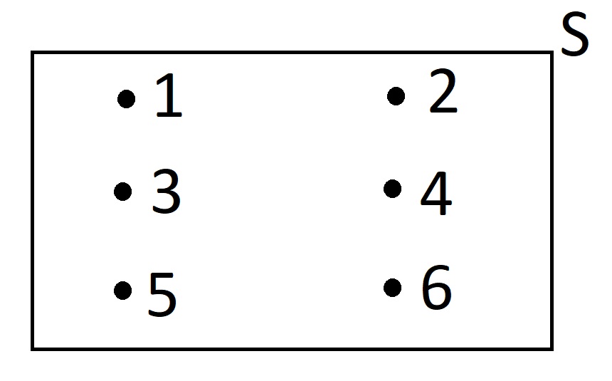
2. Rolling a regular six-sided die is an experiment where \( S = \{ 1, 2, 3, 4, 5, 6 \} \).
3. Drawing a single card from a regular deck of 52 cards is also an experiment. Why?
4. Measuring the amount of time in seconds it takes for your phone's battery life is also an experiment. What do you think the sample space is for this experiment?

When it comes to probability, having a visual aide is helpful. For that reason, we typically sketch out the sample space of a problem. Often, we will sketch out the sample space by a rectangular box labeled \( S \) and we will list out the elements in \( S \). For instance, the sample space mentioned in Example 1 and 2 above can be depicted as this:

 

 

 

 

 

 

 

Informally speaking, we will often study a set contained within a larger set which. We call this set which is contained in the larger set a subset.

Definition: Subset

Given two sets, \(A\) and \(B \), we say \(A\) is a subset of \(B\) and write \(A \subseteq B \) provided that every element of \(A\) is an element of \(B \). That is, \[ A \subseteq B \text{ if and only if } x \in A \implies x \in B \]

Example of a subset \(\PageIndex{5}\)

If \(E = \{ 1, 2 \} \) and \(S = \{ 1, 2, 3, 4, 5, 6 \} \) then \(E \subseteq S \).

Visually, we have the following:

Nonexample of a subset \(\PageIndex{6}\)

If \(A = \{ 1, 2 , 3, 4, 5 \} \) and \(B= \{ 2, 3, 4, 5, 6 \} \) then \(A \not\subseteq B \). Can you explain why?

In many cases, we will be studying the subset of a sample space and thus we reserve a special name for this set.

Definition: Event

Any subset, \(E\), of a sample space \(S\), is called an event.

Example of events \(\PageIndex{7}\)

1. If \(S = \{H, T \} \) and \(E = \{ \text{H} \} \) then \( E \) is an event since \(E \subseteq S \).
2. If \(S = \{ 1, 2, 3, 4, 5, 6 \} \) and \( E = \{ \text{we get a positive even number less than or equal to 6} \} = \{ 2, 4, 6 \} \) then \( E \subseteq S \).
3. Suppose an experiment is selecting a card at random from a regular deck of 52 cards. Then \( S = \{ \text{2 of Hearts}, \text{2 of Diamonds}, \text{2 of Clubs}, \text{2 of Spades}, \ldots, \text{Ace of Hearts}, \text{Ace of Diamonds}, \text{Ace of Clubs}, \text{Ace of Spades} \} \). If \( E = \{ \text{5 of Hearts}, \text{5 of Diamonds}, \text{5 of Clubs}, \text{5 of Spades} \}\) then \( E \subseteq S\).

For us, we will be using the words set and event interchangeably. More importantly, there is an algebra we can define on sets. What do we mean by this? Well, simply put, in the same way we can have rules for performing operations on numbers (like addition, subtraction, multiplication, and division) we can instead create rules for performing operations on sets (like taking their union, intersection, or complement).

Definition: Union, Intersection, Empty Set, Disjoint/Mutually Exclusive

For any two events, \(E\) and \(F\) of a sample space \(S\), we define \(E \cup F\), read as "\(E\) union \(F\) " to be the event which consists of all outcomes that are in either \(E\), or \(F\), or in both \(E\) and \(F\). That is,

\[ E \cup F = \{x \in S: x \in E \text{ or } x \in F\} \]

We define \(E \cap F\), read as "\(E\) intersect F\) ", to be the event which consists of all outcomes that are in both \(E\) and \(F\). That is,

\[ E \cap F = \{x \in S: x \in E \text{ and } x \in F\}\]

It should be noted that in the case that \(E\) and \(F\) share no common outcomes, we write \(E \cap F\) = \emptyset\), read as "\(E\) intersect F\) equals the empty set", where \(\emptyset\) refers to the set which contains no elements. If \(E \cap F\) = \emptyset\), then we say that \(E\) and \(F\) are disjoint or mutually exclusive events.

Examples of union and intersections \(\PageIndex{8}\)

Find \(E \cup F \) and \( E \cap F \) for each of the following examples:

1. \(E = \{ 0, 1, 2, 3, 4 \} \) and \(F = \{ 3, 4, 5, 6, 10 \} \).
2. \(E = \{ 1, 2, 3 \} \) and \(F = \{ 4, 5, 6 \} \).

Answer

1. \( E \cup F = \{0, 1, 2, 3, 4, 5, 6, 10 \} \) and \( E \cap F = \{ 3, 4 \} \).
2. \( E \cup F = \{ 1, 2, 3, 4, 5, 6 \} \) and \( E \cap F = \emptyset \).

Note

Informally, we can think of the set theoretic operation of union as "merging" the sets into one "larger" set. Meanwhile, the set theoretic operation of intersection only takes what is common or shared from the underlying sets.

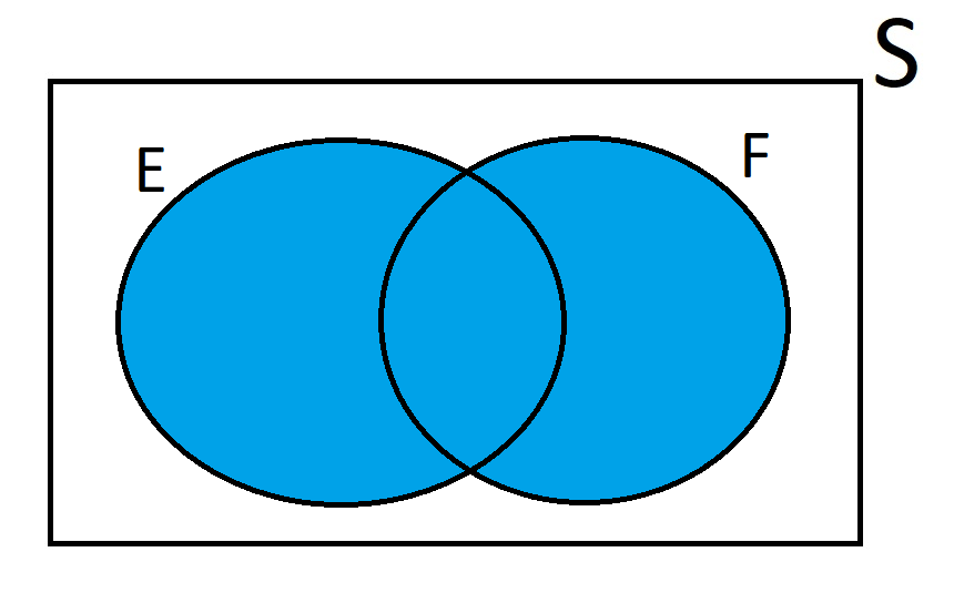
To understand these operations from a visual perspective, we can draw a Venn diagram. Here is what the Venn diagram may look like for two events:

For the above figure, can you shade the region that is referred to when we say \( E \cup F \)? Can you shade the region that is referred to when we say \( E \cap F \)?

 

 

 

 

 

 

 

 

 

 

 

If two events are disjoint, then the Venn diagram might look like the following:

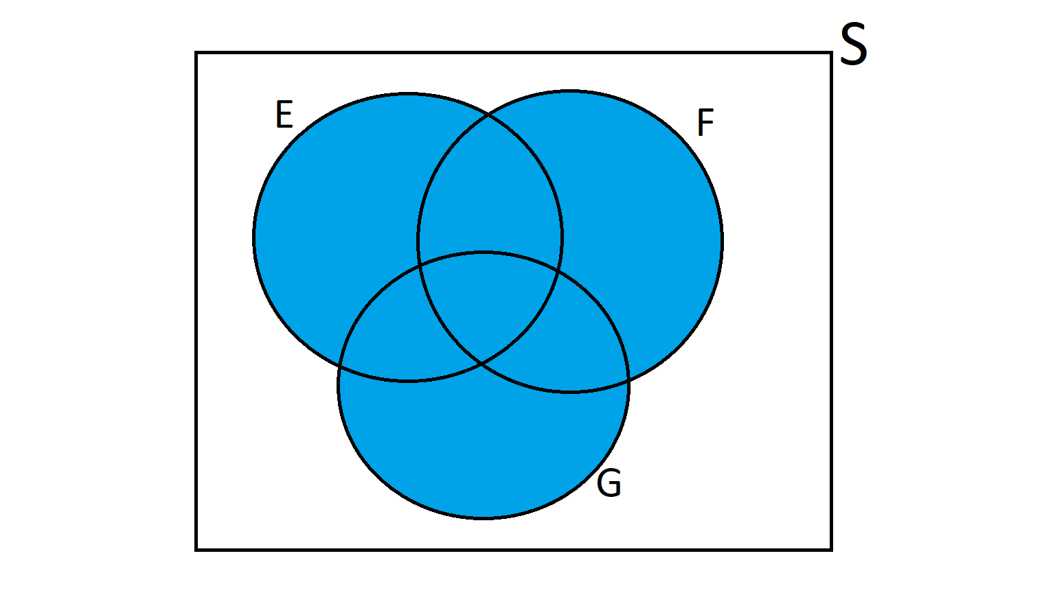
We shall now take a small jump. You see, there is no reason to restrict ourselves to studying the union or intersection of only two events. Instead, we may discuss the union or intersection of three events or four events or five events or \( k \) events. In fact, we can also have the union or intersection of infinitely many events. In terms of a Venn Diagram, let us see what is meant by the union of three events and the intersection of three events.

Example \(\PageIndex{9}\)

A Venn diagram for three events, \( E, F \) and \(G \) may look like the following:

1. Shade in \( E \cup F \cup G \).
2. Shade in \( E \cap F \cap G \).

Answer

1. 
2. 

Unfortunately, we cannot draw a picture to illustrate what it means to take the union of an infinite number of sets nor can we draw the picture for what it means to take the intersection of an infinite number of sets. Why is that? Well clearly, we cannot draw an infinite number of sets! And since we do not have a concise way of doing so, we can only present it's definition.

Definition: Countably Infinite Union of Events

If \( E_1, E_2, E_3, \ldots \) are events in a sample space \( S \), then the union of these events, denoted by
\[
\bigcup_{i=1}^{\infty} E_i = E_1 \cup E_2 \cup E_3 \cup \ldots
\]
is defined to be the event that consist of all outcomes that are in \(E_n \) for at least one value of \( n = 1, 2, 3, \ldots \). That is,

\[
\bigcup_{i=1}^{\infty} E_i = \{ x \in S ~|~ x \in E_{i} ~ \text{for some} ~ i \in \mathbb{N} \}
\]

Definition: Countably Infinite Intersection of Events

If \( E_1, E_2, E_3, \ldots \) are events in a sample space \( S \), then the intersection of these events, denoted by
\[
\bigcap_{i=1}^{\infty} E_i = E_1 \cap E_2 \cap E_3 \cap \ldots
\]
is defined to be the event that consist of all outcomes that are common to all of the events \( E_n \) for \( n = 1, 2, 3, \ldots \).

That is,

\[
\bigcap_{i=1}^{\infty} E_i = \{ x \in S ~|~ x \in E_{i} ~ \text{for all} ~ i \in \mathbb{N} \}
\]

Finally, there is one last set theoretic operation we must discuss - how to take the complement of an event.

Definition: Complement

Given any event \(A\) of a sample space \(S\), we define the complement of \(A \), denoted by \( A^c \) or \( A' \), to be the event containing all of the elements in \(S\) that are not in \(A\). That is, \[ A^c = \{ x \in S: x \notin A\} \]

Example of Complement \(\PageIndex{10}\)

Find \(E^c \) for each of the following examples:

1. \( S = \{0, 1, 2, 3, 4, 5, 6, 10 \} \) and \( E = \{ 0, 1, 2, 3 \} \)
2. \( S = \{ 1, 2, 3, 4, 5, 6 \} \) and if \( E = \{ 2, 4, 6 \} \)
3. \( S = \{ 1, 2, 3 \} \) and \( E = \{ 1, 2, 3 \} \)

Answer

1. \( E^c = \{ 4, 5, 6, 10 \} \)
2. \( E^c = \{1, 3, 5 \} \)
3. \( E^c = \emptyset \)

Exercise \(\PageIndex{11}\)

Shade in \(E^c \) on the following Venn Diagram.

Answer

We now discuss three definitions which will play a critical part in developing our theory of probability. The first definition generalizes what it means for more than two sets to be mutually exclusive. The remaining two definitions will play a central role in Week 5 when we discuss conditional probabilities.

Definition: Mutually Exclusive Events, Exhaustive Events, Forms a Partition on \( S \)

1. The events \(E_1, E_2, \ldots, E_k\) are said to be mutually exclusive events if \( E_i \cap E_j = \emptyset \) for all \(i \neq j \).
2. The events \(E_1, E_2, \ldots, E_k\) are said to be exhaustive on \(S\) if \(E_1 \cup E_2 \cup \ldots \cup E_k = S\).
3. The events \(E_1, E_2, \ldots, E_k\) are said to form a partition on \(S\)} if \(E_1, E_2, \ldots, E_k\) are mutually exclusive events and exhaustive events.

Example \(\PageIndex{12}\)

1. If \( S = \{ 1, 2, 3, 4, 5, 6 \} \) and \(E_1 = \{ 1, 2, 3 \} \) and \(E_2 = \{ 4, 5, 6 \} \) then \(E_1 \) and \(E_2 \) are disjoint or mutually exclusive.
2. If \( S = \{ 1, 2, 3, 4, 5, 6 \} \) and \(E_1 = \{ 1, 2, 3 \} \) and \(E_2 = \{ 4, 5, 6 \} \) then \(E_1 \) and \(E_2 \) are exhaustive events.
3. If \( S = \{ 1, 2, 3, 4, 5, 6 \} \) and \(E_1 = \{ 1, 2, 3 \}\) and \(E_2 = \{ 4, 5, 6 \}\) then \(E_1\) and $\(E_2\) form a partition on \(S \).
4. If \( S = \{ 1, 2, 3, 4, 5, 6 \} \) and \(E_1 = \{ 1, 2 \}\) and \(E_2 = \{ 3, 4 \}\) and \(E_3 = \{ 5, 6 \}\) then \(E_1\), \(E_2\), \(E_3\) forms a partition on \(S\).
5. If \( E_1 = \{ 1, 2, 3 \} \) and \(E_2 = \{ 4, 5, 6 \}\) and \(E_3 = \{ 7, 8, 9 \}\) then \(E_1\), \(E_2\) and \(E_3\) are said to be disjoint or mutually exclusive.
6. If \( E_1 = \{ 1, 2, 3 \} \) and \(E_2 = \{ 4, 5, 6 \}\) and \(E_3 = \{ 6, 7, 8, 9 \}\) then \(E_1\), \(E_2\) and \(E_3\) are NOT disjoint.
7. If \( S = \{ 1, 2, 3, 4, 5, 6 \} \) and \(E_1 = \{ 1, 2, 3, 4 \}\) and \(E_2 = \{ 4, 5, 6 \}\) then \(E_1\) and \(E_2\) are still exhaustive events.

Finally, we end this section with a list of theorems concerning basic set theory. A good idea is to convince yourself of the truth of each statement.

Theorem \(\PageIndex{13}\)

\(\emptyset \subseteq A\) for every set \(A\).

Proof

Answer

\( \emptyset \subseteq A \) means that \( x \in \emptyset \implies x \in A \). Since the premise is false, the implication is true.

Theorem \(\PageIndex{14}\)

Suppose that \(A\), \(B\) and \(C\) are subsets of a set \(S\). Then

1. \(A \subseteq A\) (the reflexive property).
2. If \(A \subseteq B\) and \(B \subseteq A\) then \(A = B \) (the anti-symmetric property).
3. If \(A \subseteq B\) and \(B \subseteq C\) then \(A \subseteq C\) (the transitive property).

Theorem \(\PageIndex{15}\)

If \( E \subseteq F \) then \( F = E \cup (E^c \cap F) \)

Theorem: Identity Laws \(\PageIndex{16}\)

1. \(A \cup \emptyset = A\)
2. \(A \cap S = A\)

Theorem: Idempotent Laws \(\PageIndex{17}\)

1. \(A \cup A = A\)
2. \(A \cap A = A\)

Theorem: Domination Laws \(\PageIndex{18}\)

1. \(A \cup \emptyset = A\)
2. \(A \cap \emptyset = \emptyset \)

Theorem: Complement Laws \(\PageIndex{19}\)

1. \(A \cup A^c = S\)
2. \(A \cap A^c = \emptyset\)

Theorem: Double Complement Law \(\PageIndex{20}\)

\((A^c)^c = A\)

Theorem: Commutative Laws \(\PageIndex{21}\)

1. \(A \cup B = B \cup A\)
2. \(A \cap B = B \cap A\)

Theorem: Associative Laws \(\PageIndex{22}\)

1. \(A \cup (B \cup C) = (A \cup B) \cup C\)
2. \(A \cap (B \cap C) = (A \cap B) \cap C\)

Theorem: Distributive Laws \(\PageIndex{23}\)

1. \(A \cap (B \cup C) = (A \cap B) \cup (A \cap C)\)
2. \(A \cup (B \cap C) = (A \cup B) \cap (A \cup C)\)

Theorem: Basic DeMorgans Laws \(\PageIndex{24}\)

1. \((A \cup B)^c = A^c \cap B^c\)
2. \((A \cap B)^c = A^c \cup B^c\).

Theorem: Generalized DeMorgans Laws \(\PageIndex{25}\)

1. \[ \left(\bigcup_{i =1}^{\infty} A_i \right)^c = \bigcap_{i=1}^{\infty} A_i^c \]
2. \[ \left( \bigcap_{i =1}^{\infty} A_i \right)^c = \bigcup_{i=1}^{\infty} A_i^c \]