6.1: Conditional Probabilities

↵

The topic of conditional probabilities is one of the core concepts used in machine learning. As usual, we take a motivated approach towards this new topic and show how it relates to our theory that we have discussed so far.

In the last section, we formally proved that for any event \(E\) of a simple sample space \(S\) that \[ P(E) = \frac{|E|}{|S|} \nonumber \]

Our goal is to now use this formula to motivate the answer to a rather deep question. Before we state this question allow us to be a little bit informal and abuse notation for the sake of intuition.

When we say for that a simple sample space \(S\), \[ P(E) = \frac{|E|}{|S|} \nonumber \] we are informally saying that

\[ P(A) = \frac{|E|}{|S|} = \frac{ \text{all the ``stuff" in E that can occur} }{ \text{all the ``stuff" which can possibly happen} } \nonumber \]

In fact, even when you are not in a simple sample space, the same idea holds. Notice that

\[ P(E) = \frac{P(E)}{P(S)} = \frac{ \text{all the ``stuff" in E that can occur} }{ \text{all the ``stuff" which can possibly happen} } \nonumber \]

With this idea in mind, let us consider the following question: have you ever played the MegaMillions before?

If not, then let us take a look at the following webpage: https://www.megamillions.com/How-to-Play.aspx

According to this webpage, the MegaMillions is played according to the following rules: there are two machines where Machine 1 contains 70 white balls, numbered 1 through 70, and Machine 2 contains 25 golden balls numbered 1 through 25. From Machine 1, five white balls are selected at random, one at a time, without replacement. From Machine 2, a single golden ball is selected. If a player is able to guess which five white balls are selected (in any order), and the player is able to guess which golden ball is selected, then they win the jackpot. According to the website, the probability that we win the jackpot (for a single ticket) is \( \frac{1}{302,575,350} \). Is this number accurate? Let us find out.

Example 1 \(\PageIndex{1}\)

There are two machines where Machine 1 contains 70 white balls, numbered 1 through 70, and Machine 2 contains 25 golden balls numbered 1 through 25. From Machine 1, five white balls are selected at random, one at a time, without replacement. From Machine 2, a single golden ball is selected. If a player is able to guess which five white balls are selected (in any order), and the player is able to guess which golden ball is selected, then they win the jackpot. Suppose you play a single ticket. What is the probability that you win the jackpot?

Solution

Let \(A = \{ \text{we win the jackpot} \} = \{ \text{our lottery numbers were drawn} \} \).

Let \(S\) denote the set of all possible outcomes where an outcome is a subset of the 5 white balls drawn paired with a single golden ball.

Since the selection happens at random, \(S\) is a simple sample space.

\( |S| = \binom{70}{5} \times \binom{25}{1} = 302,575,350 \).

Since we only played a single ticket, \( |A| = 1 \).

Hence \( P(A) = \frac{1}{302,575,350} \).

Hence the number reported on the webpage is indeed accurate. Observe that the above computation shows us that there is a small chance that we win the lottery. Hence, initially, the probability we win the lottery is nonzero.

For concreteness, let us suppose that on our lottery ticket, we said that the white balls numbered 24, 32, 55, 19 and 12 will be selected and the golden ball will be 17.

While watching the lottery drawing live, the first white ball that is drawn is numbered 1.

What is the probability that we win the jackpot now?

Answer

0.

The reason why is because 1 appears on the winning ticket. Since 1 does not appear on our ticket, then it means we did not win the lottery. Notice that after learning some information, the probability we win the lottery is zero.

Reflecting back on the situation we see that before \( P(A) > 0 \). However, after learning some new information that we will label by \(B\), the \( P(A ~ \text{GIVEN} ~ B ) = 0 \). That is, the presence of new information affected the probability of \(A\).

For this particular example, the effect that \(B\) had on the probability of \(A\) was obvious. However, for other situations, it may not be so clear on how to update/change/revise the probability of \(A\). For these situations, we would like to develop a formula which tells us how the probability of \(A\) changes in the presence of new information \(B\). And so the deep question that we will pose is: how can we update the the probability of \(A\) given that some other event, \(B\), has occurred ?

Allow us to informally answer this deep question by abusing notation.

As mentioned above,

\[ P(E) = \frac{P(E)}{P(S)} = \frac{ \text{all the ``stuff" in E that can occur} }{ \text{all the ``stuff" which can possibly happen} } \nonumber \]

This means

\[ P(A ~\text{given} ~ B) = \frac{ \text{all the ``stuff" in A that can occur} }{ \text{all the ``stuff" which can possibly happen} } \label{conditional} \]

In order to identify the numerator and denominator, we will consider the following diagram:

Let us first tackle the denominator of Equation \ref{conditional} . When we say \( P(A ~\text{given} ~ B) \), we are saying that the event \( B \) has happened. That is, anything outside of \(B\) cannot occur. This means all the ``stuff" which can possibly happen is precisely B.

Since \( B \) represents the set of all possibilities, \(B\) plays the role of our new (reduced) sample space.

We will now study the numerator of Equation \ref{conditional}. The numerator is all the "stuff" in \(A\) that can happen. Given that our new sample space is \(B\), in order for \(A\) to occur, we must be in the following region:

That is, given that \(B\) has occurred, in order for \(A\) to occur, we must be in \(A \cap B \). Putting everything together, we obtain the following:

\[ P(A ~\text{given} ~ B) = \frac{ \text{all the ``stuff" in A that can occur} }{ \text{all the ``stuff" which can possibly happen} } = \frac{P(A \cap B)}{P(B)} \label{conditional2} \]

Thus, we have answered the question of how the presence of new information \(B\) changes the probability of \(A\) and we take this to be our definition of a conditional probability.

Definition: The Conditional Probability

Suppose that we learn an event \(B\) has occurred and we wish to compute the probability of another event \(A\) taking into account the occurrence of \(B\). The new probability of \(A\) is called the conditional probability of the event \(A\) given that the event \(B\) has occurred and is denoted by \( P(A | B )\) which is read as "the probability of \(A\) given \(B\)". If \(P(B) > 0 \), then we compute this probability as

\[ P(A | B) = \frac{P(A \cap B)}{P(B)} \]

Example 2 \(\PageIndex{2}\)

Suppose two fair dice are rolled. Given that the first dice landed on a "3", what is the probability that a sum of 5 is obtained?

Answer

We are asked to find the probability that a sum of 5 is obtained after learning that the first dice landed on a "3". To answer this question, we will let \(A = \{ \text{the sum is a 5}\} \) and we will let \(B = \{ \text{the first dice is a 3}\} \). By our definition of conditional probability, we know that

\[ P(A | B) = \frac{P(A \cap B)}{P(B)} \nonumber \]

To complete this problem, we need to find two probabilities. We must compute \( P(A \cap B) \) and \(P(B)\). Let us first tackle the denominator, \(P(B)\).

The denominator is asking us to find the probability that the first dice lands on a 3. Recall that the experiment is that two fair dice are rolled. From the previous section, we recognize that the sample space of this experiment is a simple sample space. That is, the sample space can be thought of as the set of all outcomes where an outcome is an ordered pair. The first entry in the ordered pair denotes the outcome of rolling Die 1 and the second entry in the ordered pair denotes the outcome of rolling Die 2. Notice that \(S\) is a simple sample space because there is no reason to believe that a certain ordered pair is more likely than another ordered pair since the dice are fair. Visually we can list out the outcomes in \(S\) via the following chart:

	Die 2	1	2	3	4	5	6
Die 1
1		(1,1)	(1,2)	(1,3)	(1,4)	(1,5)	(1,6)
2		(2,1)	(2,2)	(2,3)	(2,4)	(2,5)	(2,6)
3		(3,1)	(3,2)	(3,3)	(3,4)	(3,5)	(3,6)
4		(4,1)	(4,2)	(4,3)	(4,4)	(4,5)	(4,6)
5		(5,1)	(5,2)	(5,3)	(5,4)	(5,5)	(5,6)
6		(6,1)	(6,2)	(6,3)	(6,4)	(6,5)	(6,6)

Hence \( P(B) = \frac{|B|}{|S|} = \frac{6}{36} \).

Similarly, the numerator, \( P(A \cap B) = \frac{|A \cap B| }{|S|} \).

To find \( |A \cap B| \), we ask ourselves how many outcomes belong to \(A \cap B ~ \) ? That is, how many outcomes correspond to a sum of 5 where the first die lands on a 3? The only such outcome is (3,2). Hence, \( P(A \cap B) = \frac{|A \cap B| }{|S|} = \frac{1}{36} \).

Putting everything together yields

\[ P(A | B) = \frac{P(A \cap B)}{P(B)} = \frac{ \frac{|A \cap B|}{|S|} }{ \frac{|B|}{|S|} }= \frac{ \frac{1}{36} }{\frac{6}{36}} = \frac{1}{6} \nonumber \]

While this completes the problem, notice that before, \(P(A) = 4/36 \). After learning the event \(B\) has taken place, \( P(A|B) = \frac{1}{6} = \frac{6}{36} \). Thus, learning that \(B\) has occured has made \(A\) more likely to occur.

Example 2 \(\PageIndex{3}\)

Suppose two fair dice are rolled. Given that the sum of the two dice is 5, what is the probability that the first dice lands on a 3?

Answer

For convenience, let us stick to the notation that we used in Example 1. We will let \(A = \{ \text{the sum is a 5}\} \) and \(B = \{ \text{the first dice is a 3}\} \). We are now asked to find \( P(B|A) \). By a similar argument to the above problem, \[ P(B | A) = \frac{P(B \cap A)}{P(A)} = \frac{ \frac{|B \cap A|}{|S|} }{ \frac{|A|}{|S|} }= \frac{ \frac{1}{36} }{\frac{4}{36}} = \frac{1}{4} \nonumber \]

While this completes the problem, notice that before, \(P(B) = \frac{6}{36} = \frac{1}{6} \). After learning the event \(A\) has taken place, \( P(B|A) = \frac{1}{4} = \frac{9}{36} \). Thus, learning that \(A\) has occured has made \(B\) more likely to occur.

Before we consider the next example, allow us to make an observation. In the lottery example, we saw that \(P(A) > P(A|B) \). In the example above, we saw that \( P(A) < P(A|B) \).

Hence, the presence of new information \(B\) can either increase the probability of \(A\) (as in the dice example) or decrease the probability of \(A\) (as in the lottery example). However, there is a third case we may wish to consider. Namely, is it possible that some new information \(B\) can have no affect on the probability of \(A\)? Allow us to consider the following example which will answer this question. (Note: You should highlight this problem since it will be the central focus in the next section!).

Example \(\PageIndex{4}\)

Suppose a card is selected at random from a regular deck of cards. Let \( E = \{ \text{the selected card is an ace} \} \) and let \( F = \{ \text{the selected card is a spade} \} \). Find \(P(E), P(F), P(E|F) \) and \(P(F|E) \).

Answer

Since the card is selected at random, we are in a simple sample space. Hence \(P(E) = \frac{|E|}{|S|} = \frac{4}{52} = \frac{1}{13} \). By a similar argument, \(P(F) = \frac{|F|}{|S|} = \frac{13}{52} = \frac{1}{4} \).

To find \( P(E|F) \), we simply note that

\[ P( E | F ) = \frac{P(E \cap F)}{P(F)} = \frac{ \frac{|E \cap F|}{|S|} }{ \frac{|F|}{|S|} }= \frac{ \frac{1}{52} }{\frac{13}{52}} = \frac{1}{13} \nonumber \]

Notice that \( P(E) = P(E|F) \).

Meanwhile, to find \( P(F|E) \), we simply note that

\[ P( F | E ) = \frac{P(F \cap E)}{P(E)} = \frac{ \frac{|F \cap E|}{|S|} }{ \frac{|E|}{|S|} }= \frac{ \frac{1}{52} }{\frac{4}{52}} = \frac{1}{4} \nonumber \]

Notice that \( P(F) = P(F|E) \).

Allow us to make a comment regarding the above problem as to why it is trivial that \(P(E) = \( P(E|F) \). Suppose that we were playing a game where you draw a card at random and if that card is an ace, then you would win the game. Before you draw your card, the probability that you get an ace is \( \frac{4}{52} = \frac{1}{13} \).

Suppose after you selected a face down card, I take a quick peek at the card and inform you that the card you drew was a spade. Does this new knowledge about the selected card affect the probability of you winning? Not at all! You see, with the knowledge that the card is a spade, you know that the card has thirteen possibilities. Of these thirteen possibilities, only one of them is an ace and since all of these outcomes are equally likely, the probability that the card is an ace is \( \frac{1}{13} \) which is precisely our initial probability.

Note that we can perform a similar analysis to explain why \( P(F) = P(F|E) \).

Theorem \(\PageIndex{5}\)

Theorem: Suppose \(B\) is an event of sample space \(S\) such that \(P(B)>0\). Then for any event \(A\) in \(S\), \[ P(A^c | B) = 1 - P(A|B) \nonumber \]

Proof:

Let as an exercise to the reader.

Theorem: The Basic Conditioning Rule \(\PageIndex{6}\)

Theorem: Suppose \(A\) and \(B\) are events in a sample space \(S\).

1. If \(P(A) > 0\), then \( P(A \cap B) = P(A) P(B|A) \).
2. If \(P(B) > 0\), then \( P(A \cap B) = P(B) P(A|B) \).

Proof:

We only show the proof of (1) as the proof of (2) is similar.

Consider the expression \( P(A) P(B|A) \). Substituting the definition of \( P(B|A) \) into \( P(A) P(B|A) \) yields the following:

\begin{align*} P(A) P(B|A) &= P(A) \times \frac{P(B \cap A)}{P(A)} \\ &= P(B \cap A) \\ &= P(A \cap B) \end{align*}

Notice the above result tells us that we have a choice to make when studying an intersection. Whenever we are dealing with \( P(A \cap B) \), we must decide if we wish to rewrite this as \( P(A) P(B|A) \) or as \( P(B) P(A|B) \). How do we know which one to select? The answer is that it will depend either on the experiment or the probabilities available to us within the problem.

Example \(\PageIndex{7}\)

Suppose an urn has 10 red marbles and 6 blue marbles. An experiment consists of drawing two marbles from the bowl, one at a time without replacement. If we assume at each draw, each marble is equally likely to be chosen, then find the probability that both marbles are red. (Try this problem on your own before reading our solution!).

Answer

We will answer this question in two different ways.

Solution 1: In our first solution, we stick to the counting framework introduced in Section 4.1. Let \( A = \{ \text{both marbles are red} \} \). Let \(S\) denote the set of all outcomes where an outcome is a subset of two marbles. \(S\) is a simple sample space since there is no reason to believe that a certain subset of two marbles is more likely than another subset of two marbles. \(|S| = \binom{16}{2} \) while \( |A| = \binom{10}{2} \). Putting everything together, we see that

\[ P(A) = \frac{|A|}{|S|} = \frac{\binom{10}{2} }{\binom{16}{2}} = 0.375 \nonumber\ \]

Solution 2: Recall from Section 2.1 that we said in rephrasing an event, it may be helpful to ask ourselves "can we describe this event by using the words or/and?"

For us, \( A = \{ \text{both marbles are red} \} \) can be rephrased as \( A = \{ \text{marble 1 is red and marble 2 is red} \} \). In order to introduce suitable notation to describe \(A\), we define \( R_i = \{ \text{marble} ~ i ~ \text{is red} \} \). Thus, \(A = R_1 \cap R_2 \). This gives us the following:

\[ P(A) = P(R_1 \cap R_2) = P(R_1) P(R_2 | R_1) \nonumber\ \]

Note that our starting configuration looks like this:

Clearly, \( P(R_1) = \frac{10}{16} \). To find \( P(R_2 | R_1) \), we note that given \(R_1\), our new bowl looks like this:

And so given that \(R_1\) has occurred, we now face the above composition. Hence the probability of \(R_2 \) with respect to our new sample space is given by \( \frac{9}{15} \). Putting everything together, we see that

\[ P(A) = P(R_1 \cap R_2) = P(R_1) P(R_2 | R_1) = \frac{10}{16} \times \frac{9}{15} = 0.375 \nonumber\ \]

The Basic Conditioning Rule tells us how to deal with the probability of an intersection of two events. However, there is no reason to limit ourselves to studying the intersection of only two events. Instead, we may wish to deal with the intersection of three or four or in general, \(k\) events. To do so, we use The Generalized Conditioning Rule.

Theorem: The Generalized Conditioning Rule \(\PageIndex{8}\)

Theorem: Suppose that \( A_1, A_2, A_3, \ldots, A_n \) are events in a sample space \(S\) such that \( P(A_1 \cap A_2 \cap A_3 \cap \ldots \cap A_{n-1} > 0 \). Then

\[ P(P(A_1 \cap A_2 \cap A_3 \cap \ldots \cap A_{n} ) = P(A_1) P(A_2 | A_1) P(A_3 | A_1 \cap A_2) \ldots P(A_n | A_1 \cap A_2 \cap \ldots \cap A_{n-1} ) \]

Proof

Let as an exercise to the reader.

Example \(\PageIndex{9}\)

Suppose an urn has 10 red marbles and 6 blue marbles. An experiment consists of drawing three marbles from the bowl, one at a time without replacement. If we assume at each draw, each marble is equally likely to be chosen, then find the probability that the first two marbles are red and the third marble is blue.

Answer

Let \( A = \{ \text{the first two marbles are red and the third marble is blue} \} \). We can rephrase this event as \( A = \{ \text{marble 1 is red and marble 2 is red and marble 3 is blue} \} \). In order to introduce suitable notation to describe \(A\), we define \( R_i = \{ \text{marble} ~ i ~ \text{is red} \} \) and \( B_i = \{ \text{marble} ~ i ~ \text{is blue} \} \). Thus, \(A = R_1 \cap R_2 \cap B_3 \). This gives us the following:

\[ P(A) = P(R_1 \cap R_2 \cap B_3) = P(R_1) P(R_2 | R_1) P(B_3 | R_1 \cap R_2) \nonumber\ \]

Note that our starting configuration looks like this:

Clearly, \( P(R_1) = \frac{10}{16} \). To find \( P(R_2 | R_1) \), we note that given \(R_1\), our new bowl looks like this:

And so given that \(R_1\) has occurred, we now face the above composition. Hence the probability of \(R_2 \) with resepct to our new sample space is given by \( \frac{9}{15} \).

Similarly, to find \( P(B_3 | R_1 \cap R_2 \) we note that given \(R_1 \cap R_2 \), our new bowl looks like this:

And so given that \(R_1 \cap R_2 \), has occurred, we now face the above composition. Hence the probability of \(B_3 \) with respect to the newest sample space is \( \frac{6}{14} \).

Putting everything together, we see that

\[ P(A) = P(R_1 \cap R_2 \cap B_3) = P(R_1) P(R_2 | R_1) P(B_3 | R_1 \cap R_2) \nonumber\ = \frac{10}{16} \times \frac{9}{15} \times \frac{6}{14} \approx 0.1607 \nonumber\ \]

Example \(\PageIndex{10}\)

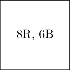
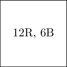
Suppose an urn has 10 red marbles and 6 blue marbles. An experiment consists of drawing three marbles from the bowl, one at a time. Suppose each time a marble is selected from the bowl, the selected marble is replaced along with two additional marbles of the same color. If we assume at each draw, each marble is equally likely to be chosen, then find the probability that the first two marbles are red and the third marble is blue.

Answer

Let \( A = \{ \text{the first two marbles are red and the third marble is blue} \} \). We can rephrase this event as \( A = \{ \text{marble 1 is red and marble 2 is red and marble 3 is blue} \} \). In order to introduce suitable notation to describe \(A\), we define \( R_i = \{ \text{marble} ~ i ~ \text{is red} \} \) and \( B_i = \{ \text{marble} ~ i ~ \text{is blue} \} \). Thus, \(A = R_1 \cap R_2 \cap B_3 \). This gives us the following:

\[ P(A) = P(R_1 \cap R_2 \cap B_3) = P(R_1) P(R_2 | R_1) P(B_3 | R_1 \cap R_2) \nonumber\ \]

Note that our starting configuration looks like this:

Clearly, \( P(R_1) = \frac{10}{16} \). To find \( P(R_2 | R_1) \), we note that given \(R_1\), our new bowl looks like this:

And so given that \(R_1\) has occurred, we now face the above composition. Hence the probability of \(R_2 \) with resepct to our new sample space is given by \( \frac{12}{18} \).

Similarly, to find \( P(B_3 | R_1 \cap R_2 \) we note that given \(R_1 \cap R_2 \), our new bowl looks like this:

And so given that \(R_1 \cap R_2 \), has occurred, we now face the above composition. Hence the probability of \(B_3 \) with respect to the newest sample space is \( \frac{6}{20} \).

Putting everything together, we see that

\[ P(A) = P(R_1 \cap R_2 \cap B_3) = P(R_1) P(R_2 | R_1) P(B_3 | R_1 \cap R_2) \nonumber\ = \frac{10}{16} \times \frac{12}{18} \times \frac{6}{20} \approx 0.125 \nonumber\ \]