1.3: Rates of Change and Behavior of Graphs

Last updated
Save as PDF

Page ID: 117098

$ \newcommand{\vecs}[1]{\overset { \scriptstyle \rightharpoonup} {\mathbf{#1}} } $ $ \newcommand{\vecd}[1]{\overset{-\!-\!\rightharpoonup}{\vphantom{a}\smash {#1}}} $$\newcommand{\id}{\mathrm{id}}$ $ \newcommand{\Span}{\mathrm{span}}$ $ \newcommand{\kernel}{\mathrm{null}\,}$ $ \newcommand{\range}{\mathrm{range}\,}$ $ \newcommand{\RealPart}{\mathrm{Re}}$ $ \newcommand{\ImaginaryPart}{\mathrm{Im}}$ $ \newcommand{\Argument}{\mathrm{Arg}}$ $ \newcommand{\norm}[1]{\| #1 \|}$ $ \newcommand{\inner}[2]{\langle #1, #2 \rangle}$ $ \newcommand{\Span}{\mathrm{span}}$ $\newcommand{\id}{\mathrm{id}}$ $ \newcommand{\Span}{\mathrm{span}}$ $ \newcommand{\kernel}{\mathrm{null}\,}$ $ \newcommand{\range}{\mathrm{range}\,}$ $ \newcommand{\RealPart}{\mathrm{Re}}$ $ \newcommand{\ImaginaryPart}{\mathrm{Im}}$ $ \newcommand{\Argument}{\mathrm{Arg}}$ $ \newcommand{\norm}[1]{\| #1 \|}$ $ \newcommand{\inner}[2]{\langle #1, #2 \rangle}$ $ \newcommand{\Span}{\mathrm{span}}$$\newcommand{\AA}{\unicode[.8,0]{x212B}}$

Finding the Average Rate of Change of a Function

The price change per year is a rate of change because it describes how an output quantity changes relative to the change in the input quantity. We can see that the price of gasoline in Table $\PageIndex{1}$ did not change by the same amount each year, so the rate of change was not constant. If we use only the beginning and ending data, we would be finding the average rate of change over the specified period of time. To find the average rate of change, we divide the change in the output value by the change in the input value.

\[\begin{align*} \text{Average rate of change}&=\dfrac{\text{Change in output}}{\text{Change in input}} \\[4pt] &=\dfrac{\Delta y}{\Delta x}\\[4pt] &=\dfrac{y_2-y_1}{x_2-x_1}\\[4pt] &=\dfrac{f(x_2)-f(x_1)}{x_2-x_1}\end{align*} \label{1.3.1}\]

The Greek letter $\Delta$ (delta) signifies the change in a quantity; we read the ratio as “delta-$y$ over delta-$x$” or “the change in $y$ divided by the change in $x$.” Occasionally we write $\Delta f$ instead of $\Delta y$, which still represents the change in the function’s output value resulting from a change to its input value. It does not mean we are changing the function into some other function.

In our example, the gasoline price increased by $1.37 from 2005 to 2012. Over 7 years, the average rate of change was

\[\dfrac{\Delta y}{\Delta x}=\dfrac{$1.37}{7 \text{years}}\approx \text{0.196 dollars per year.} \label{1.3.2}\]

On average, the price of gas increased by about 19.6¢ each year. Other examples of rates of change include:

A population of rats increasing by 40 rats per week
A car traveling 68 miles per hour (distance traveled changes by 68 miles each hour as time passes)
A car driving 27 miles per gallon (distance traveled changes by 27 miles for each gallon)
The current through an electrical circuit increasing by 0.125 amperes for every volt of increased voltage
The amount of money in a college account decreasing by $4,000 per quarter

Definition: Rate of Change

A rate of change describes how an output quantity changes relative to the change in the input quantity. The units on a rate of change are “output units per input units.”

The average rate of change between two input values is the total change of the function values (output values) divided by the change in the input values.

\[\dfrac{\Delta y}{\Delta x}=\dfrac{f(x_2)-f(x_1)}{x_2-x_1}\]

Figure $\PageIndex{5}$: Definition of a local maximum

These observations lead us to a formal definition of local extrema.

Local Minima and Local Maxima

A function $f$ is an increasing function on an open interval if $f(b)>f(a)$ for every $a$, $b$ interval where $b>a$.
A function $f$ is a decreasing function on an open interval if $f(b)<f(a)$ for every $a$, $b$ interval where $b>a$.

A function $f$ has a local maximum at a point $b$ in an open interval $(a,c)$ if $f(b)$ is greater than or equal to $f(x)$ for every point $x$ ($x$ does not equal $b$) in the interval. Likewise, $f$ has a local minimum at a point $b$ in $(a,c)$ if $f(b)$ is less than or equal to $f(x)$ for every $x$ ($x$ does not equal $b$) in the interval.

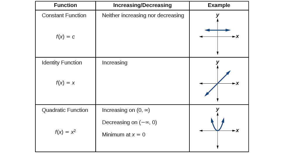
Analyzing the Toolkit Functions for Increasing or Decreasing Intervals

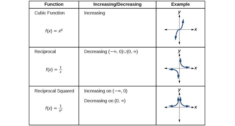
We will now return to our toolkit functions and discuss their graphical behavior in Figure $\PageIndex{10}$, Figure $\PageIndex{11}$, and Figure $\PageIndex{12}$.

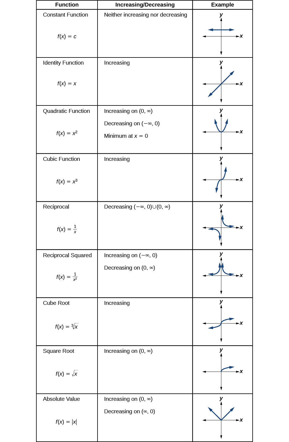
$Table showing the increasing and decreasing intervals of the toolkit functions.$
Figure $\PageIndex{12}$

Use A Graph to Locate the Absolute Maximum and Absolute Minimum

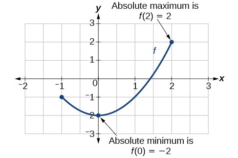
There is a difference between locating the highest and lowest points on a graph in a region around an open interval (locally) and locating the highest and lowest points on the graph for the entire domain. The y-coordinates (output) at the highest and lowest points are called the absolute maximum and absolute minimum, respectively. To locate absolute maxima and minima from a graph, we need to observe the graph to determine where the graph attains it highest and lowest points on the domain of the function (Figure $\PageIndex{13}$).

Figure $\PageIndex{13}$: Graph of a segment of a parabola with an absolute minimum at (0, -2) and absolute maximum at (2, 2).

Not every function has an absolute maximum or minimum value. The toolkit function $f(x)=x^3$ is one such function.

Absolute Maxima and Minima

The absolute maximum of $f$ at $x=c$ is $f(c)$ where $f(c)≥f(x)$ for all $x$ in the domain of $f$.
The absolute minimum of $f$ at $x=d$ is $f(d)$ where $f(d)≤f(x)$ for all $x$ in the domain of $f$.