2.2: Graphs of Linear Functions
- Page ID
- 117108

Graphing Linear Functions
Previously, we saw that that the graph of a linear function is a straight line. We were also able to see the points of the function as well as the initial value from a graph. By graphing two functions, then, we can more easily compare their characteristics. There are three basic methods of graphing linear functions:
- Plot the points and then drawing a line through the points.
- Use the y-intercept and slope.
- Use transformations of the identity function \(f(x)=x\).
Graphing a Function by Plotting Points
To find points of a function, we can choose input values, evaluate the function at these input values, and calculate output values. The input values and corresponding output values form coordinate pairs. We then plot the coordinate pairs on a grid. In general, we should evaluate the function at a minimum of two inputs in order to find at least two points on the graph. For example, given the function, \(f(x)=2x\), we might use the input values 1 and 2. Evaluating the function for an input value of 1 yields an output value of 2, which is represented by the point \((1,2)\). Evaluating the function for an input value of 2 yields an output value of 4, which is represented by the point \((2,4)\). Choosing three points is often advisable because if all three points do not fall on the same line, we know we made an error.
- Choose a minimum of two input values.
- Evaluate the function at each input value.
- Use the resulting output values to identify coordinate pairs.
- Plot the coordinate pairs on a grid.
- Draw a line through the points.
Graph \(f(x)=−\frac{2}{3}x+5\) by plotting points.
Solution
Begin by choosing input values. This function includes a fraction with a denominator of 3, so let’s choose multiples of 3 as input values. We will choose 0, 3, and 6.
Evaluate the function at each input value, and use the output value to identify coordinate pairs.
\[\begin{align*} x&=0 & f(0)&=-\dfrac{2}{3}(0)+5=5\rightarrow(0,5) \\ x&=3 & f(3)&=-\dfrac{2}{3}(3)+5=3\rightarrow(3,3) \\ x&=6 & f(6)&=-\dfrac{2}{3}(6)+5=1\rightarrow(6,1) \end{align*}\]
Plot the coordinate pairs and draw a line through the points. Figure \(\PageIndex{1}\) represents the graph of the function \(f(x)=−\frac{2}{3}x+5\).
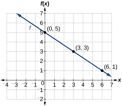
Analysis
The graph of the function is a line as expected for a linear function. In addition, the graph has a downward slant, which indicates a negative slope. This is also expected from the negative constant rate of change in the equation for the function.
Graph \(f(x)=−\frac{3}{4}x+6\) by plotting points.
- Answer
-
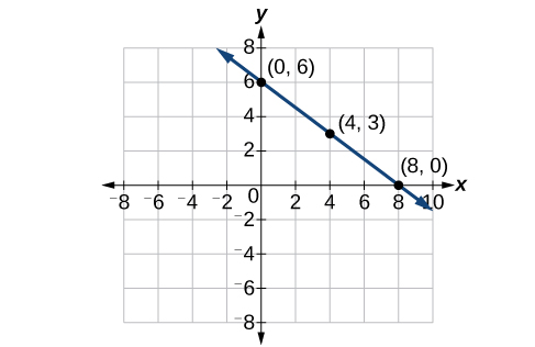
Figure \(\PageIndex{2}\)
Graphing a Function Using y-intercept and Slope
Another way to graph linear functions is by using specific characteristics of the function rather than plotting points. The first characteristic is its y-intercept, which is the point at which the input value is zero. To find the y-intercept, we can set \(x=0\) in the equation.
The other characteristic of the linear function is its slope \(m\), which is a measure of its steepness. Recall that the slope is the rate of change of the function. The slope of a function is equal to the ratio of the change in outputs to the change in inputs. Another way to think about the slope is by dividing the vertical difference, or rise, by the horizontal difference, or run. We encountered both the y-intercept and the slope in Linear Functions.
Let’s consider the following function.
\[f(x)=\dfrac{1}{2}x+1\]
The slope is \(\frac{1}{2}\). Because the slope is positive, we know the graph will slant upward from left to right. The y-intercept is the point on the graph when \(x=0\). The graph crosses the y-axis at \((0,1)\). Now we know the slope and the y-intercept. We can begin graphing by plotting the point \((0,1)\) We know that the slope is rise over run, \(m=\frac{\text{rise}}{\text{run}}\). From our example, we have \(m=\frac{1}{2}\), which means that the rise is 1 and the run is 2. So starting from our y-intercept \((0,1)\), we can rise 1 and then run 2, or run 2 and then rise 1. We repeat until we have a few points, and then we draw a line through the points as shown in Figure \(\PageIndex{3}\).
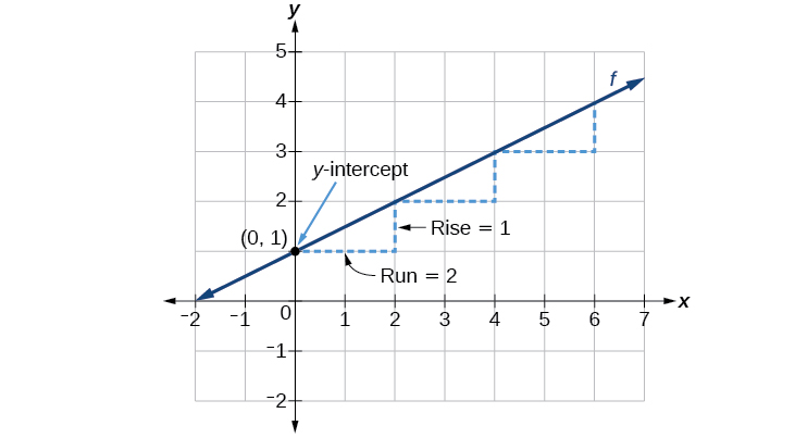
In the equation \(f(x)=mx+b\)
- \(b\) is the y-intercept of the graph and indicates the point \((0,b)\) at which the graph crosses the y-axis.
- \(m\) is the slope of the line and indicates the vertical displacement (rise) and horizontal displacement (run) between each successive pair of points. Recall the formula for the slope:
\[m=\dfrac{\text{change in output (rise)}}{\text{change in input (run)}}=\dfrac{{\Delta}y}{{\Delta}x}=\dfrac{y_2-y_1}{x_2-x_1}\]
Graphing a Function Using Transformations
Another option for graphing is to use transformations of the identity function \(f(x)=x\). A function may be transformed by a shift up, down, left, or right. A function may also be transformed using a reflection, stretch, or compression.
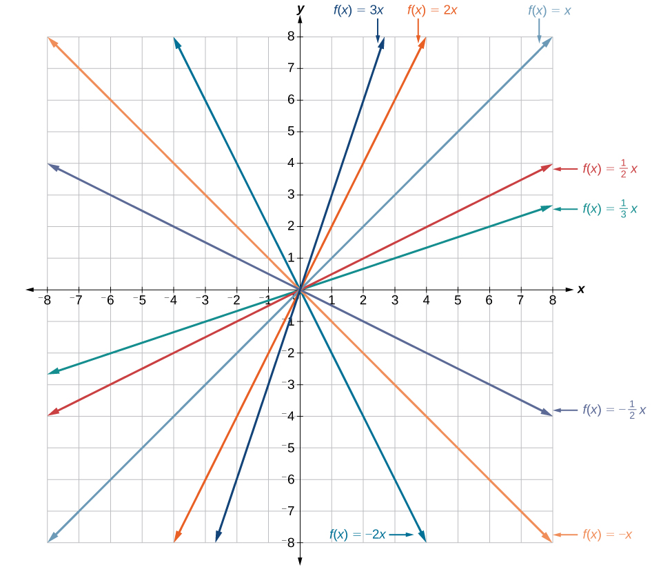
Vertical Stretch or Compression
In the equation \(f(x)=mx\), the \(m\) is acting as the vertical stretch or compression of the identity function. When \(m\) is negative, there is also a vertical reflection of the graph. Notice in Figure \(\PageIndex{5}\) that multiplying the equation of \(f(x)=x\) by \(m\) stretches the graph of \(f\) by a factor of \(m\) units if \(m>1\) and compresses the graph of \(f\) by a factor of \(m\) units if \(0
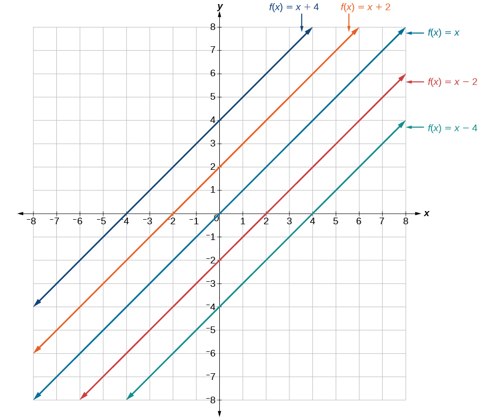
Vertical Shift
In \(f(x)=mx+b\), the \(b\) acts as the vertical shift, moving the graph up and down without affecting the slope of the line. Notice in Figure \(\PageIndex{6}\) that adding a value of \(b\) to the equation of \(f(x)=x\) shifts the graph of \(f\) a total of \(b\) units up if \(b\) is positive and \(|b|\) units down if \(b\) is negative.
Using vertical stretches or compressions along with vertical shifts is another way to look at identifying different types of linear functions. Although this may not be the easiest way to graph this type of function, it is still important to practice each method.
Describing Horizontal and Vertical Lines
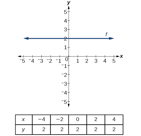
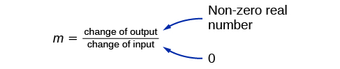
There are two special cases of lines on a graph—horizontal and vertical lines. A horizontal line indicates a constant output, or y-value. In Figure \(\PageIndex{15}\), we see that the output has a value of 2 for every input value. The change in outputs between any two points, therefore, is 0. In the slope formula, the numerator is 0, so the slope is 0. If we use \(m=0\) in the equation \(f(x)=mx+b\), the equation simplifies to \(f(x)=b\). In other words, the value of the function is a constant. This graph represents the function \(f(x)=2\).
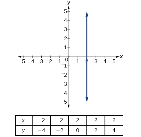
A vertical line indicates a constant input, or x-value. We can see that the input value for every point on the line is 2, but the output value varies. Because this input value is mapped to more than one output value, a vertical line does not represent a function. Notice that between any two points, the change in the input values is zero. In the slope formula, the denominator will be zero, so the slope of a vertical line is undefined.
Notice that a vertical line, such as the one in Figure \(\PageIndex{17}\), has an x-intercept, but no y-intercept unless it’s the line \(x=0\). This graph represents the line \(x=2\).
Lines can be horizontal or vertical.
- A horizontal line is a line defined by an equation in the form \(f(x)=b\).
- A vertical line is a line defined by an equation in the form \(x=a\).
Writing the Equation of a Line Parallel or Perpendicular to a Given Line
If we know the equation of a line, we can use what we know about slope to write the equation of a line that is either parallel or perpendicular to the given line.
Writing Equations of Parallel Lines
Suppose for example, we are given the following equation.
\[f(x)=3x+1 \nonumber\]
We know that the slope of the line formed by the function is 3. We also know that the y-intercept is \((0,1)\). Any other line with a slope of 3 will be parallel to \(f(x)\). So the lines formed by all of the following functions will be parallel to \(f(x)\).
\[\begin{align*} g(x)&=3x+6 \\ h(x)&=3x+1\\ p(x)&=3x+\dfrac{2}{3} \end{align*}\]
Suppose then we want to write the equation of a line that is parallel to \(f\) and passes through the point \((1, 7)\). We already know that the slope is 3. We just need to determine which value for \(b\) will give the correct line. We can begin with the point-slope form of an equation for a line, and then rewrite it in the slope-intercept form.
\[\begin{align*} y−y_1&=m(x−x_1) \\ y−7&=3(x−1) \\ y−7&=3x−3 \\ y&=3x+4 \end{align*}\]
So \(g(x)=3x+4\) is parallel to \(f(x)=3x+1\) and passes through the point \((1, 7)\).
Solving a System of Linear Equations Using a Graph
A system of linear equations includes two or more linear equations. The graphs of two lines will intersect at a single point if they are not parallel. Two parallel lines can also intersect if they are coincident, which means they are the same line and they intersect at every point. For two lines that are not parallel, the single point of intersection will satisfy both equations and therefore represent the solution to the system.
To find this point when the equations are given as functions, we can solve for an input value so that \(f(x)=g(x)\). In other words, we can set the formulas for the lines equal to one another, and solve for the input that satisfies the equation.
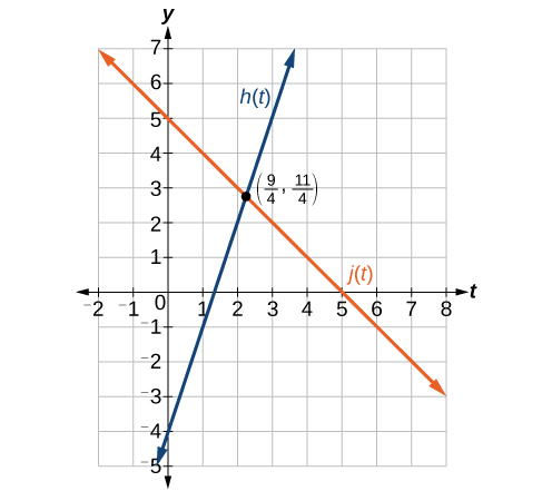
Find the point of intersection of the lines \(h(t)=3t−4\) and \(j(t)=5−t\).
Solution
Set \(h(t)=j(t)\).
\[\begin{align} 3t-4&=5-t \\ 4t&=9 \\ t&=\dfrac{9}{4} \end{align}\]
This tells us the lines intersect when the input is \(\frac{9}{4}\).
We can then find the output value of the intersection point by evaluating either function at this input.
\[\begin{align} j\Big( \dfrac{9}{4} \Big)&=5-\dfrac{9}{4} \\ &= \dfrac{11}{4}\end{align}\]
These lines intersect at the point \(\Big(\frac{9}{4},\frac{11}{4}\Big)\).
Analysis
Looking at Figure \(\PageIndex{25}\), this result seems reasonable.