
6.2: Graphs of the Other Trigonometric Functions
- Page ID
- 117148

Analyzing the Graph of \(y =\tan x\)
We will begin with the graph of the tangent function, plotting points as we did for the sine and cosine functions. Recall that
\[\tan \, x=\dfrac{\sin \, x}{\cos \, x}\]
The period of the tangent function is \(\pi\) because the graph repeats itself on intervals of \(k\pi\) where \(k\) is a constant. If we graph the tangent function on \(−\frac{\pi}{2}\) to \(\frac{\pi}{2}\), we can see the behavior of the graph on one complete cycle. If we look at any larger interval, we will see that the characteristics of the graph repeat.
We can determine whether tangent is an odd or even function by using the definition of tangent.
\[\begin{align*} \tan(-x)&= \dfrac{\sin(-x)}{\cos(-x)} \qquad \text{Definition of tangent}\\ &= \dfrac{-\sin \, x}{\cos \, x} \qquad \text{Sine is an odd function, cosine is even}\\ &= -\dfrac{\sin \, x}{\cos \, x} \qquad \text{The quotient of an odd and an even function is odd}\\ &= -\tan \, x \qquad \text{Definition of tangent} \end{align*}\]
Therefore, tangent is an odd function. We can further analyze the graphical behavior of the tangent function by looking at values for some of the special angles, as listed in Table \(\PageIndex{1}\).
| \(x\) | \(−\dfrac{\pi}{2}\) | \(−\dfrac{\pi}{3}\) | \(−\dfrac{\pi}{4}\) | \(−\dfrac{\pi}{6}\) | 0 | \(\dfrac{\pi}{6}\) | \(\dfrac{\pi}{4}\) | \(\dfrac{\pi}{3}\) | \(\dfrac{\pi}{2}\) |
|---|---|---|---|---|---|---|---|---|---|
| \(\tan x\) | undefined | \(-\sqrt{3}\) | \(–1\) | \(-\dfrac{\sqrt{3}}{3}\) | 0 | \(\dfrac{\sqrt{3}}{3}\) | 1 | \(\sqrt{3}\) | undefined |
These points will help us draw our graph, but we need to determine how the graph behaves where it is undefined. If we look more closely at values when \(\frac{\pi}{3}<x<\frac{\pi}{2}\), we can use a table to look for a trend. Because \(\frac{\pi}{3}≈1.05\) and \(\frac{\pi}{2}≈1.57\), we will evaluate \(x\) at radian measures \(1.05<x<1.57\) as shown in Table \(\PageIndex{2}\).
| \(x\) | 1.3 | 1.5 | 1.55 | 1.56 |
|---|---|---|---|---|
| \(\tan x\) | 3.6 | 14.1 | 48.1 | 92.6 |
As \(x\) approaches \(\dfrac{\pi}{2}\), the outputs of the function get larger and larger. Because \(y=\tan \, x\) is an odd function, we see the corresponding table of negative values in Table \(\PageIndex{3}\).
| \(x\) | −1.3 | −1.5 | −1.55 | −1.56 |
|---|---|---|---|---|
| \(\tan x\) | −3.6 | −14.1 | −48.1 | −92.6 |
We can see that, as \(x\) approaches \(−\frac{\pi}{2}\), the outputs get smaller and smaller. Remember that there are some values of \(x\) for which \(\cos \, x=0\). For example, \(\cos \left (\frac{\pi}{2} \right)=0\) and \(\cos \left (\frac{3\pi}{2} \right )=0\). At these values, the tangent function is undefined, so the graph of \(y=\tan \, x\) has discontinuities at \(x=\frac{\pi}{2}\) and \(\frac{3\pi}{2}\). At these values, the graph of the tangent has vertical asymptotes. Figure \(\PageIndex{1}\) represents the graph of \(y=\tan \, x\). The tangent is positive from \(0\) to \(\frac{\pi}{2}\) and from \(\pi\) to \(\frac{3\pi}{2}\), corresponding to quadrants I and III of the unit circle.
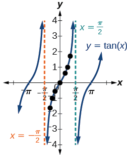
Figure \(\PageIndex{1}\): Graph of the tangent function
Graphing Variations of \(y = \tan \, x\)
As with the sine and cosine functions, the tangent function can be described by a general equation.
\[y=A\tan(Bx) \nonumber\]
We can identify horizontal and vertical stretches and compressions using values of \(A\) and \(B\). The horizontal stretch can typically be determined from the period of the graph. With tangent graphs, it is often necessary to determine a vertical stretch using a point on the graph.
Because there are no maximum or minimum values of a tangent function, the term amplitude cannot be interpreted as it is for the sine and cosine functions. Instead, we will use the phrase stretching/compressing factor when referring to the constant \(A\).
- The stretching factor is \(|A|\).
- The period is \(P=\dfrac{\pi}{|B|}\).
- The domain is all real numbers \(x\),where \(x≠\dfrac{\pi}{2| B |}+\dfrac{π}{| B |}k\) such that \(k\) is an integer.
- The range is \((−\infty,\infty)\).
- The asymptotes occur at \(x=\dfrac{\pi}{2| B |}+\dfrac{π}{| B |}k\) where \(k\) is an integer.
- \(y=A\tan(Bx)\) is an odd function.
Graphing One Period of a Stretched or Compressed Tangent Function
We can use what we know about the properties of the tangent function to quickly sketch a graph of any stretched and/or compressed tangent function of the form \(f(x)=A\tan(Bx)\). We focus on a single period of the function including the origin, because the periodic property enables us to extend the graph to the rest of the function’s domain if we wish. Our limited domain is then the interval \(\left (−\dfrac{P}{2},\dfrac{P}{2} \right )\) and the graph has vertical asymptotes at \(\pm \dfrac{P}{2}\) where \(P=\dfrac{\pi}{B}\). On \(\left (−\dfrac{\pi}{2},\dfrac{\pi}{2} \right )\), the graph will come up from the left asymptote at \(x=−\dfrac{\pi}{2}\), cross through the origin, and continue to increase as it approaches the right asymptote at \(x=\dfrac{\pi}{2}\). To make the function approach the asymptotes at the correct rate, we also need to set the vertical scale by actually evaluating the function for at least one point that the graph will pass through. For example, we can use
\[f \left (\dfrac{P}{4} \right )=A\tan \left (B\dfrac{P}{4} \right )=A\tan \left (B\dfrac{\pi}{4B} \right )=A \nonumber\]
because \(\tan \left (\dfrac{\pi}{4} \right )=1\).
- Identify the stretching factor, \(| A |\).
- Identify B and determine the period, \(P=\dfrac{\pi}{| B |}\).
- Draw vertical asymptotes at \(x=−\dfrac{P}{2}\) and \(x=\dfrac{P}{2}\).
- For \(A>0\), the graph approaches the left asymptote at negative output values and the right asymptote at positive output values (reverse for \(A<0\)).
- Plot reference points at \(\left (\dfrac{P}{4},A \right )\), \((0,0)\), and \(\left (−\dfrac{P}{4},−A \right )\), and draw the graph through these points.
Graphing One Period of a Shifted Tangent Function
Now that we can graph a tangent function that is stretched or compressed, we will add a vertical and/or horizontal (or phase) shift. In this case, we add \(C\) and \(D\) to the general form of the tangent function.
\[f(x)=A\tan(Bx−C)+D \nonumber\]
The graph of a transformed tangent function is different from the basic tangent function \(\tan x\) in several ways:
- The stretching factor is \(| A |\).
- The period is \(\dfrac{\pi}{| B |}\).
- The domain is \(x≠\dfrac{C}{B}+\dfrac{\pi}{| B |}k\),where \(k\) is an integer.
- The range is \((−∞,−| A |]∪[| A |,∞)\).
- The vertical asymptotes occur at \(x=\dfrac{C}{B}+\dfrac{\pi}{| B |}k\),where \(k\) is an odd integer.
- There is no amplitude.
- \(y=A \tan(Bx)\) is and odd function because it is the qoutient of odd and even functions(sin and cosine perspectively).
- Express the function given in the form \(y=A\tan(Bx−C)+D\).
- Identify the stretching/compressing factor, \(| A |\).
- Identify \(B\) and determine the period, \(P=\dfrac{\pi}{|B|}\).
- Identify \(C\) and determine the phase shift, \(\dfrac{C}{B}\).
- Draw the graph of \(y=A\tan(Bx)\) shifted to the right by \(\dfrac{C}{B}\) and up by \(D\).
- Sketch the vertical asymptotes, which occur at \(x=\dfrac{C}{B}+\dfrac{\pi}{2| B |}k\),where \(k\) is an odd integer.
- Plot any three reference points and draw the graph through these points.
Analyzing the Graphs of \(y = \sec x\) and \(y = \csc x\)
The secant was defined by the reciprocal identity \(sec \, x=\dfrac{1}{\cos x}\). Notice that the function is undefined when the cosine is \(0\), leading to vertical asymptotes at \(\dfrac{\pi}{2}\), \(\dfrac{3\pi}{2}\) etc. Because the cosine is never more than \(1\) in absolute value, the secant, being the reciprocal, will never be less than \(1\) in absolute value.
We can graph \(y=\sec x\) by observing the graph of the cosine function because these two functions are reciprocals of one another. See Figure \(\PageIndex{8}\). The graph of the cosine is shown as a dashed orange wave so we can see the relationship. Where the graph of the cosine function decreases, the graph of the secant function increases. Where the graph of the cosine function increases, the graph of the secant function decreases. When the cosine function is zero, the secant is undefined.
The secant graph has vertical asymptotes at each value of \(x\) where the cosine graph crosses the \(x\)-axis; we show these in the graph below with dashed vertical lines, but will not show all the asymptotes explicitly on all later graphs involving the secant and cosecant.
Note that, because cosine is an even function, secant is also an even function. That is, \(\sec(−x)=\sec x\).
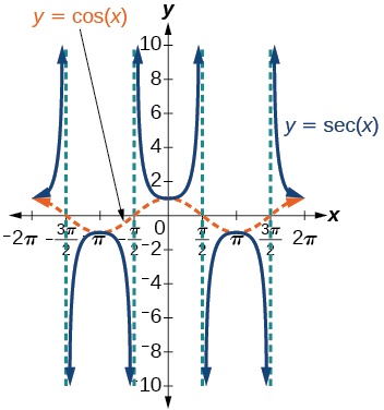
Figure \(\PageIndex{8}\): Graph of the secant function, \(f(x)=\sec x=\dfrac{1}{\cos x}\)
As we did for the tangent function, we will again refer to the constant \(| A |\) as the stretching factor, not the amplitude.
- The stretching factor is \(| A |\).
- The period is \(\dfrac{2\pi}{| B |}\).
- The domain is \(x≠\dfrac{\pi}{2| B |}k\), where \(k\) is an odd integer.
- The range is \((−∞,−|A|]∪[|A|,∞)\).
- The vertical asymptotes occur at \(x=\dfrac{\pi}{2| B |}k\), where \(k\) is an odd integer.
- There is no amplitude.
- \(y=A\sec(Bx)\) is an even function because cosine is an even function.
Similar to the secant, the cosecant is defined by the reciprocal identity \(\csc x=\dfrac{1}{\sin x}\). Notice that the function is undefined when the sine is \(0\), leading to a vertical asymptote in the graph at \(0\), \(\pi\), etc. Since the sine is never more than \(1\) in absolute value, the cosecant, being the reciprocal, will never be less than \(1\) in absolute value.
We can graph \(y=\csc x\) by observing the graph of the sine function because these two functions are reciprocals of one another. See Figure \(\PageIndex{7}\). The graph of sine is shown as a dashed orange wave so we can see the relationship. Where the graph of the sine function decreases, the graph of the cosecant function increases. Where the graph of the sine function increases, the graph of the cosecant function decreases.
The cosecant graph has vertical asymptotes at each value of \(x\) where the sine graph crosses the \(x\)-axis; we show these in the graph below with dashed vertical lines.
Note that, since sine is an odd function, the cosecant function is also an odd function. That is, \(\csc(−x)=−\csc x\).
The graph of cosecant, which is shown in Figure \(\PageIndex{9}\), is similar to the graph of secant.
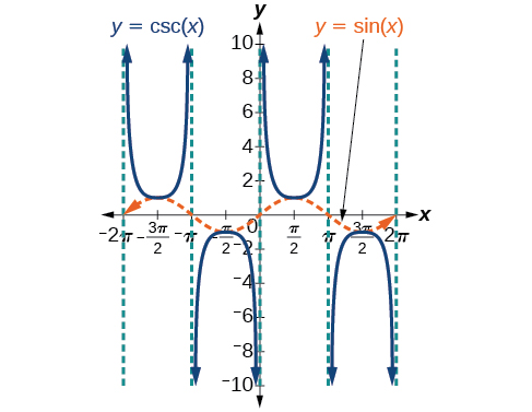
Figure \(\PageIndex{9}\): The graph of the cosecant function, \(f(x)=\csc x=\frac{1}{\sin x}\)
- The stretching factor is \(| A |\).
- The period is \(\dfrac{2\pi}{|B|}\).
- The domain is \(x≠\dfrac{\pi}{|B|}k\), where \(k\) is an integer.
- The range is \((−∞,−|A|]∪[|A|,∞)\).
- The asymptotes occur at \(x=\dfrac{\pi}{| B |}k\), where \(k\) is an integer.
- \(y=A\csc(Bx)\) is an odd function because sine is an odd function.
Graphing Variations of \(y = \sec x\) and \(y= \csc x\)
For shifted, compressed, and/or stretched versions of the secant and cosecant functions, we can follow similar methods to those we used for tangent and cotangent. That is, we locate the vertical asymptotes and also evaluate the functions for a few points (specifically the local extrema). If we want to graph only a single period, we can choose the interval for the period in more than one way. The procedure for secant is very similar, because the cofunction identity means that the secant graph is the same as the cosecant graph shifted half a period to the left. Vertical and phase shifts may be applied to the cosecant function in the same way as for the secant and other functions.The equations become the following.
\[y=A\sec(Bx−C)+D\]
\[y=A\csc(Bx−C)+D\]
- The stretching factor is \(|A|\).
- The period is \(\dfrac{2\pi}{|B|}\).
- The domain is \(x≠\dfrac{C}{B}+\dfrac{\pi}{2| B |}k\),where \(k\) is an odd integer.
- The range is \((−∞,−|A|]∪[|A|,∞)\).
- The vertical asymptotes occur at \(x=\dfrac{C}{B}+\dfrac{π}{2| B |}k\),where \(k\) is an odd integer.
- There is no amplitude.
- \(y=A\sec(Bx)\) is an even function because cosine is an even function.
- The stretching factor is \(|A|\).
- The period is \(\dfrac{2\pi}{|B|}\).
- The domain is \(x≠\dfrac{C}{B}+\dfrac{\pi}{2| B |}k\),where \(k\) is an integer.
- The range is \((−∞,−|A|]∪[|A|,∞)\).
- The vertical asymptotes occur at \(x=\dfrac{C}{B}+\dfrac{\pi}{|B|}k\),where \(k\) is an integer.
- There is no amplitude.
- \(y=A\csc(Bx)\) is an odd function because sine is an odd function.
- Express the function given in the form \(y=A\sec(Bx)\).
- Identify the stretching/compressing factor, \(|A|\).
- Identify \(B\) and determine the period, \(P=\dfrac{2\pi}{| B |}\).
- Sketch the graph of \(y=A\cos(Bx)\).
- Use the reciprocal relationship between \(y=\cos \, x\) and \(y=\sec \, x\) to draw the graph of \(y=A\sec(Bx)\).
- Sketch the asymptotes.
- Plot any two reference points and draw the graph through these points.
Analyzing the Graph of \(y = \cot x\)
The last trigonometric function we need to explore is cotangent. The cotangent is defined by the reciprocal identity \(cot \, x=\dfrac{1}{\tan x}\). Notice that the function is undefined when the tangent function is \(0\), leading to a vertical asymptote in the graph at \(0\), \(\pi\), etc. Since the output of the tangent function is all real numbers, the output of the cotangent function is also all real numbers.
We can graph \(y=\cot x\) by observing the graph of the tangent function because these two functions are reciprocals of one another. See Figure \(\PageIndex{19}\). Where the graph of the tangent function decreases, the graph of the cotangent function increases. Where the graph of the tangent function increases, the graph of the cotangent function decreases.
The cotangent graph has vertical asymptotes at each value of \(x\) where \(\tan x=0\); we show these in the graph below with dashed lines. Since the cotangent is the reciprocal of the tangent, \(\cot x\) has vertical asymptotes at all values of \(x\) where \(\tan x=0\), and \(\cot x=0\) at all values of \(x\) where \(\tan x\) has its vertical asymptotes.
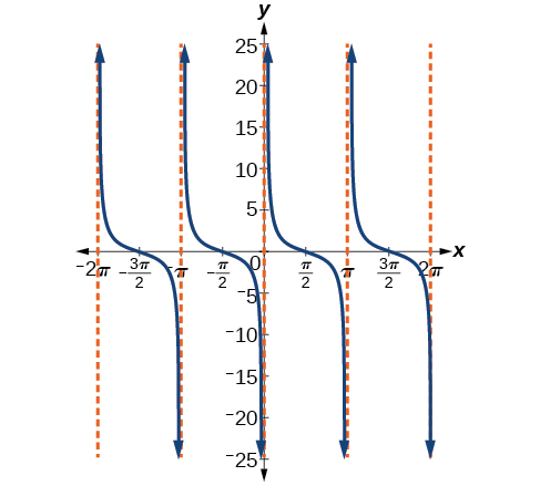
Figure \(\PageIndex{19}\): The cotangent function
- The stretching factor is \(|A|\).
- The period is \(P=\dfrac{\pi}{|B|}\).
- The domain is \(x≠\dfrac{\pi}{|B|}k\), where \(k\) is an integer.
- The range is \((−∞,∞)\).
- The asymptotes occur at \(x=\dfrac{\pi}{| B |}k\), where \(k\) is an integer.
- \(y=A\cot(Bx)\) is an odd function.
Using the Graphs of Trigonometric Functions to Solve Real-World Problems
Many real-world scenarios represent periodic functions and may be modeled by trigonometric functions. As an example, let’s return to the scenario from the section opener. Have you ever observed the beam formed by the rotating light on a police car and wondered about the movement of the light beam itself across the wall? The periodic behavior of the distance the light shines as a function of time is obvious, but how do we determine the distance? We can use the tangent function.
Suppose the function \(y=5\tan(\dfrac{\pi}{4}t)\) marks the distance in the movement of a light beam from the top of a police car across a wall where \(t\) is the time in seconds and \(y\) is the distance in feet from a point on the wall directly across from the police car.
- Find and interpret the stretching factor and period.
- Graph on the interval \([0,5]\).
- Evaluate \(f(1)\) and discuss the function’s value at that input.
Solution
- We know from the general form of \(y=A\tan(Bt)\) that \(| A |\) is the stretching factor and \(\dfrac{\pi}{B}\) is the period.
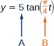
Figure \(\PageIndex{22}\)
We see that the stretching factor is \(5\). This means that the beam of light will have moved \(5\) ft after half the period.
The period is \(\dfrac{\pi}{\tfrac{\pi}{4}}=\dfrac{\pi}{1}⋅\dfrac{4}{\pi}=4\). This means that every \(4\) seconds, the beam of light sweeps the wall. The distance from the spot across from the police car grows larger as the police car approaches.
- To graph the function, we draw an asymptote at \(t=2\) and use the stretching factor and period. See Figure \(\PageIndex{23}\)
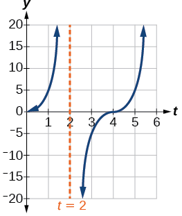
Figure \(\PageIndex{23}\)
- period: \(f(1)=5\tan(\frac{\pi}{4}(1))=5(1)=5\); after \(1\) second, the beam of has moved \(5\) ft from the spot across from the police car.