8.6: Parametric Equations

Parameterizing a Curve

When an object moves along a curve—or curvilinear path—in a given direction and in a given amount of time, the position of the object in the plane is given by the \(x\)-coordinate and the \(y\)-coordinate. However, both \(x\) and \(y\) vary over time and so are functions of time. For this reason, we add another variable, the parameter, upon which both \(x\) and \(y\) are dependent functions. In the example in the section opener, the parameter is time, \(t\). The \(x\) position of the moon at time, \(t\), is represented as the function \(x(t)\), and the \(y\) position of the moon at time, \(t\), is represented as the function \(y(t)\). Together, \(x(t)\) and \(y(t)\) are called parametric equations, and generate an ordered pair \((x(t), y(t))\). Parametric equations primarily describe motion and direction.

When we parameterize a curve, we are translating a single equation in two variables, such as \(x\) and \(y\),into an equivalent pair of equations in three variables, \(x\), \(y\), and \(t\). One of the reasons we parameterize a curve is because the parametric equations yield more information: specifically, the direction of the object’s motion over time.

When we graph parametric equations, we can observe the individual behaviors of \(x\) and of \(y\). There are a number of shapes that cannot be represented in the form \(y=f(x)\), meaning that they are not functions. For example, consider the graph of a circle, given as \(r^2=x^2+y^2\). Solving for \(y\) gives \(y=\pm \sqrt{r^2−x^2}\), or two equations: \(y_1=\sqrt{r^2−x^2}\) and \(y_2=−\sqrt{r^2−x^2}\). If we graph \(y_1\) and \(y_2\) together, the graph will not pass the vertical line test, as shown in Figure \(\PageIndex{2}\). Thus, the equation for the graph of a circle is not a function.

Figure \(\PageIndex{2}\)

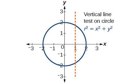
However, if we were to graph each equation on its own, each one would pass the vertical line test and therefore would represent a function. In some instances, the concept of breaking up the equation for a circle into two functions is similar to the concept of creating parametric equations, as we use two functions to produce a non-function. This will become clearer as we move forward.

PARAMETRIC EQUATIONS

Suppose \(t\) is a number on an interval, \(I\). The set of ordered pairs, \((x(t), y(t))\), where \(x=f(t)\) and \(y=g(t)\),forms a plane curve based on the parameter \(t\). The equations \(x=f(t)\) and \(y=g(t)\) are the parametric equations.

Example \(\PageIndex{1}\): Parameterizing a Curve

Parameterize the curve \(y=x^2−1\) letting \(x(t)=t\). Graph both equations.

Solution

If \(x(t)=t\), then to find \(y(t)\) we replace the variable \(x\) with the expression given in \(x(t)\). In other words, \(y(t)=t^2−1\).Make a table of values similar to Table \(\PageIndex{1}\), and sketch the graph.

Table \(\PageIndex{1}\)

\(t\)	\(x(t)\)	\(y(t)\)
\(−4\)	\(−4\)	\(y(−4)={(−4)}^2−1=15\)
\(−3\)	\(−3\)	\(y(−3)={(−3)}^2−1=8\)
\(−2\)	\(−2\)	\(y(−2)={(−2)}^2−1=3\)
\(−1\)	\(−1\)	\(y(−1)={(−1)}^2−1=0\)
\(0\)	\(0\)	\(y(0)={(0)}^2−1=−1\)
\(1\)	\(1\)	\(y(1)={(1)}^2−1=0\)
\(2\)	\(2\)	\(y(2)={(2)}^2−1=3\)
\(3\)	\(3\)	\(y(3)={(3)}^2−1=8\)
\(4\)	\(4\)	\(y(4)={(4)}^2−1=15\)

See the graphs in Figure \(\PageIndex{3}\) . It may be helpful to use the TRACE feature of a graphing calculator to see how the points are generated as \(t\) increases.

Figure \(\PageIndex{3}\): (a) Parametric \(y(t)=t^2−1\) (b) Rectangular \(y=x^2−1\)

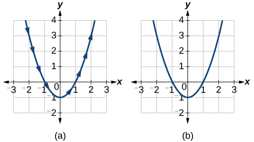
Analysis

The arrows indicate the direction in which the curve is generated. Notice the curve is identical to the curve of \(y=x^2−1\).