13.5: Constant Coefficient Equations with Piecewise Continuous Forcing Functions
- Page ID
- 121704

We’ll now consider initial value problems of the form
\[\label{eq:8.5.1} ay''+by'+cy=f(t), \quad y(0)=k_0,\quad y'(0)=k_1,\]
where \(a\), \(b\), and \(c\) are constants (\(a\ne0\)) and \(f\) is piecewise continuous on \([0,\infty)\). Problems of this kind occur in situations where the input to a physical system undergoes instantaneous changes, as when a switch is turned on or off or the forces acting on the system change abruptly.
It can be shown (Exercises 8.5.23 and 8.5.24) that the differential equation in Equation \ref{eq:8.5.1} has no solutions on an open interval that contains a jump discontinuity of \(f\). Therefore we must define what we mean by a solution of Equation \ref{eq:8.5.1} on \([0,\infty)\) in the case where \(f\) has jump discontinuities. The next theorem motivates our definition. We omit the proof.
Suppose \(a,b\), and \(c\) are constants \((a\ne0),\) and \(f\) is piecewise continuous on \([0,\infty).\) with jump discontinuities at \(t_1,\) …, \(t_n,\) where
\[0<t_1<\cdots<t_n. \nonumber\]
Let \(k_0\) and \(k_1\) be arbitrary real numbers. Then there is a unique function \(y\) defined on \([0,\infty)\) with these properties:
- \(y(0)=k_0\) and \(y'(0)=k_1\).
- \(y\) and \(y'\) are continuous on \([0,\infty)\).
- \(y''\) is defined on every open subinterval of \([0,\infty)\) that does not contain any of the points \(t_1,\) …, \(t_n\), and \[ay''+by'+cy=f(t) \nonumber\] on every such subinterval.
- \(y''\) has limits from the right and left at \(t_1,\) …\(,\) \(t_n\).
We define the function \(y\) of Theorem 13.5.1 to be the solution of the initial value problem Equation \ref{eq:8.5.1}.
We begin by considering initial value problems of the form
\[\label{eq:8.5.2} ay''+by'+cy=\left\{\begin{array}{cl} f_0(t),&0\le t<t_1,\\[4pt]f_1(t),&t\ge t_1, \end{array}\right.\quad y(0)=k_0,\quad y'(0)=k_1,\]
where the forcing function has a single jump discontinuity at \(t_1\).
We can solve Equation \ref{eq:8.5.2} by the these steps:
- Step 1. Find the solution \(y_0\) of the initial value problem \[ay''+by'+cy=f_0(t), \quad y(0)=k_0,\quad y'(0)=k_1. \nonumber \]
- Step 2. Compute \(c_0=y_0(t_1)\) and \(c_1=y_0'(t_1)\).
- Step 3. Find the solution \(y_1\) of the initial value problem \[ay''+by'+cy=f_1(t), \quad y(t_1)=c_0,\quad y'(t_1)=c_1.\nonumber\]
- Step 4. Obtain the solution \(y\) of Equation \ref{eq:8.5.2} as \[y=\left\{\begin{array}{cl} y_0(t),&0\le t<t_1\\[4pt]y_1(t),&t\ge t_1. \end{array}\right.\nonumber\]
It is shown in Exercise 8.5.23 that \(y'\) exists and is continuous at \(t_1\). The next example illustrates this procedure.
Solve the initial value problem
\[\label{eq:8.5.3} y''+y=f(t), \quad y(0)=2,\; y'(0)=-1,\]
where
\[f(t)=\left\{\begin{array}{rl} 1,&0\le t< \frac{\pi}{2},\\[4pt] -1,&t\ge \frac{\pi}{2}. \end{array}\right. \nonumber\]
Solution
The initial value problem in Step 1 is
\[y''+y=1, \quad y(0)=2,\quad y'(0)=-1. \nonumber\]
We leave it to you to verify that its solution is
\[y_0=1+\cos t-\sin t. \nonumber\]
Doing Step 2 yields \(y_0(\pi/2)=0\) and \(y_0'(\pi/2)=-1\), so the second initial value problem is
\[y''+y=-1, \quad y\left({\pi\over2}\right)=0,\; y'\left({\pi\over 2}\right)=-1. \nonumber\]
We leave it to you to verify that the solution of this problem is
\[y_1=-1+\cos t+\sin t. \nonumber\]
Hence, the solution of Equation \ref{eq:8.5.3} is
\[\label{eq:8.5.4} y=\left\{\begin{array}{rl} 1+\cos t-\sin t,&0\le t< {\pi\over2}, \\[4pt] -1+\cos t+\sin t,&t\ge {\pi\over2} \end{array}\right.\]
If \(f_0\) and \(f_1\) are defined on \([0,\infty)\), we can rewrite Equation \ref{eq:8.5.2} as
\[ay''+by'+cy=f_0(t)+u(t-t_1)\left(f_1(t)-f_0(t)\right), \quad y(0)=k_0,\quad y'(0)=k_1, \nonumber\]
and apply the method of Laplace transforms. We’ll now solve the problem considered in Example [example:8.5.1} by this method.
Use the Laplace transform to solve the initial value problem
\[\label{eq:8.5.5} y''+y=f(t), \quad y(0)=2,\; y'(0)=-1,\]
where
\[f(t)=\left \{ \begin{array}{cl} \phantom{-}1,&0\le t< \frac{\pi}{2},\\ -1,&t \ge \frac{\pi}{2}. \end{array}\right. \nonumber\]
Solution
Here
\[f(t)=1-2u\left(t-{\pi\over2}\right), \nonumber\]
so Theorem 13.5.1 (with \(g(t)=1\)) implies that
\[{\cal L}(f)={1-2e^{-{\pi s/2}}\over s}. \nonumber\]
Therefore, transforming Equation \ref{eq:8.5.5} yields
\[(s^2+1)Y(s)={1-2e^{-{\pi s/ 2}}\over s}-1+2s, \nonumber\]
so
\[\label{eq:8.5.6} Y(s)=(1-2e^{-{\pi s/ 2}}) G(s)+{2s-1\over s^2+1},\]
with
\[G(s)={1\over s(s^2+1)}. \nonumber\]
The form for the partial fraction expansion of \(G\) is
\[\label{eq:8.5.7} {1\over s(s^2+1)}={A\over s}+{Bs+C\over s^2+1}. \]
Multiplying through by \(s(s^2+1)\) yields
\[A(s^2+1)+(Bs+C)s=1, \nonumber\]
or
\[(A+B)s^2+Cs+A=1. \nonumber\]
Equating coefficients of like powers of \(s\) on the two sides of this equation shows that \(A=1\), \(B=-A=-1\) and \(C=0\). Hence, from Equation \ref{eq:8.5.7},
\[G(s)={1\over s}-{s\over s^2+1}. \nonumber\]
Therefore
\[g(t)=1-\cos t. \nonumber\]
From this, Equation \ref{eq:8.5.6}, and Theorem 8.4.2,
\[y=1-\cos t-2u\left(t-{\pi\over2}\right)\left(1-\cos\left(t-{\pi \over2}\right)\right)+2\cos t-\sin t. \nonumber\]
Simplifying this (recalling that \(\cos (t-\pi/2)=\sin t)\) yields
\[y=1+\cos t-\sin t-2u\left(t-{\pi\over2}\right)(1-\sin t), \nonumber\]
or
\[y=\left\{\begin{array}{cl}{1+\cos t-\sin t,}&{0\leq t<\frac{\pi }{2}}\\{-1+\cos t+\sin t,}&{t\geq \frac{\pi }{2}} \end{array} \right.\nonumber \]
which is the result obtained in Example 13.5.1 .
It isn’t obvious that using the Laplace transform to solve Equation \ref{eq:8.5.2} as we did in Example 13.5.2 yields a function \(y\) with the properties stated in Theorem 13.5.1 ; that is, such that \(y\) and \(y'\) are continuous on \([0, ∞)\) and \(y''\) has limits from the right and left at \(t_{1}\). However, this is true if \(f_{0}\) and \(f_{1}\) are continuous and of exponential order on \([0, ∞)\). A proof is sketched in Exercises 8.6.11–8.6.13.
Solve the initial value problem
\[\label{eq:8.5.8} y''-y=f(t), \quad y(0)=-1,\; y'(0)=2,\]
where
\[f(t)=\left\{\begin{array}{cl} t,&0\le t<1,\\ 1,&t\ge 1. \end{array}\right.\nonumber\]
Solution
Here
\[f(t)=t-u(t-1)(t-1),\nonumber\]
so
\[\begin{align*} {\cal L}(f)&={\cal L}(t)-{\cal L}\left(u(t-1)(t-1)\right)\\[4pt] &=\cal L(t)-e^{-s}{\cal L}(t) & & \text{ (from Theorem 8.4.1)}\\[4pt] &={1\over s^2}-{e^{-s}\over s^2}.\end{align*}\nonumber\]
Since transforming Equation \ref{eq:8.5.8} yields
\[(s^2-1) Y(s)={\cal L}(f)+2-s,\nonumber\]
we see that
\[\label{eq:8.5.9} Y(s)=(1-e^{-s})H(s)+{2-s\over s^2-1},\]
where
\[H(s)={1\over s^2(s^2-1)}={1\over s^2-1}-{1\over s^2};\nonumber\]
therefore
\[\label{eq:8.5.10} h(t)=\sinh t-t.\]
Since
\[{\cal L}^{-1}\left({2-s\over s^2-1}\right)=2\sinh t-\cosh t,\nonumber\]
we conclude from Equation \ref{eq:8.5.9}, Equation \ref{eq:8.5.10}, and Theorem 13.5.1 that
\[y=\sinh t-t-u(t-1)\left(\sinh (t-1)-t+1\right)+2\sinh t- \cosh t,\nonumber\]
or
\[\label{eq:8.5.11} y=3\sinh t-\cosh t-t-u(t-1)\left(\sinh (t-1)-t+1\right)\]
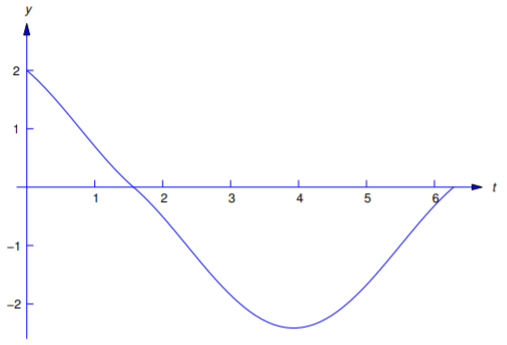
We leave it to you to verify that \(y\) and \(y'\) are continuous and \(y''\) has limits from the right and left at \(t_1=1\).
Solve the initial value problem
\[\label{eq:8.5.12} y''+y=f(t), \quad y(0)=0,\; y'(0)=0,\]
where
\[f(t)=\left\{\begin{array}{cl}{0,}&{0\leq t<\frac{\pi }{4}}\\{\cos 2t}&{\frac{\pi }{4}\leq t< \pi }\\{0,}&{t\geq \pi } \end{array} \right.\nonumber \]
Solution
Here
\[f(t)=u(t-\pi/4)\cos2t-u(t-\pi)\cos2t, \nonumber\]
so
\[\begin{align*} {\cal L}(f)&={\cal L}\left(u(t-\pi/4)\cos2t\right)-{\cal L}\left( u(t-\pi)\cos2t\right)\\[4pt] &=e^{-{\pi s/4}}{\cal L}\left(\cos2(t+\pi/4)\right)-e^{-\pi s} {\cal L}\left(\cos2(t+\pi)\right)\\[4pt] &=-e^{-{\pi s/4}}{\cal L}(\sin2t)-e^{-\pi s} {\cal L}(\cos2t)\\[4pt] &=-{2e^{-{\pi s/ 4}}\over s^2+4}-{se^{-\pi s}\over s^2+4}.\end{align*}\nonumber\]
Since transforming Equation \ref{eq:8.5.12} yields
\[(s^2+1)Y(s)={\cal L}(f),\nonumber\]
we see that
\[\label{eq:8.5.13} Y(s)=e^{-{\pi s/ 4}} H_1(s)+e^{-\pi s} H_2(s),\]
where
\[\label{eq:8.5.14} H_1(s)=-{2\over (s^2+1)(s^2+4)}\quad\mbox{ and }\quad H_2(s)=-{s \over (s^2+1)(s^2+4)}.\]
To simplify the required partial fraction expansions, we first write
\[{1\over (x+1)(x+4)}={1\over3}\left[{1\over x+1}-{1\over x+4}\right].\nonumber\]
Setting \(x=s^2\) and substituting the result in Equation \ref{eq:8.5.14} yields
\[H_1(s)=-{2\over3}\left[{1\over s^2+1}-{1\over s^2+4}\right] \quad\mbox{ and }\quad H_2(s)=-{1\over3}\left[{s\over s^2+1}-{s\over s^2+4}\right].\nonumber\]
The inverse transforms are
\[h_1(t)=-{2\over3}\sin t+{1\over3}\sin2t \quad\mbox{ and }\; h_2(t)=-{1\over3}\cos t+{1\over3}\cos2t.\nonumber\]
From Equation \ref{eq:8.5.13} and Theorem 8.4.2,
\[\label{eq:8.5.15} y=u\left(t-{\pi\over4}\right) h_1\left(t-{\pi\over4}\right)+ u(t-\pi) h_2(t-\pi).\]
Since
\[\begin{aligned} h_1\left(t-{\pi\over4}\right)&=-{2\over3}\sin\left(t-{\pi\over 4}\right)+{1\over3}\sin2\left(t-{\pi\over4}\right)\\ &=-{\sqrt{2}\over3} (\sin t-\cos t)-{1\over3}\cos2t\end{aligned}\nonumber\]
and
\[\begin{align*} h_2(t-\pi)&=-{1\over3}\cos (t-\pi)+{1\over3}\cos2(t-\pi)\\ &={1\over3}\cos t+{1\over3}\cos2t,\end{align*}\nonumber\]
Equation \ref{eq:8.5.15} can be rewritten as
\[y=-{1\over3}u\left(t-{\pi\over4}\right)\left(\sqrt{2}(\sin t-\cos t)+\cos2t\right) + {1\over3} u(t-\pi) (\cos t+\cos2t)\nonumber\]
or
\[\label{eq:8.5.16} \left\{\begin{array}{cl}{0,}&{0\leq t< \frac{\pi }{4}}\\{-\frac{\sqrt{2}}{3}(\sin t-\cos t)-\frac{1}{3}\cos 2t,}&{\frac{\pi }{4}\leq t<\pi ,}\\{-\frac{\sqrt{2}}{3}\sin t+\frac{1+\sqrt{2}}{3}\cos t,}&{t\geq\pi } \end{array} \right. \]
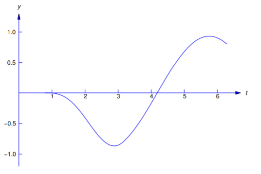
We leave it to you to verify that \(y\) and \(y'\) are continuous and \(y''\) has limits from the right and left at \(t_1=\pi/4\) and \(t_2=\pi\) (Figure 13.5.2 ).