7.2: Orthogonal Sets of Vectors

The idea that two lines can be perpendicular is fundamental in geometry, and this section is devoted to introducing this notion into a general inner product space \(V\). To motivate the definition, recall that two nonzero geometric vectors \(\mathbf{x}\) and \(\mathbf{y}\) in \(\mathbb{R}^{n}\) are perpendicular (or orthogonal) if and only if \(\mathbf{x} \cdot \mathbf{y}=0\). In general, two vectors \(\mathbf{v}\) and \(\mathbf{w}\) in an inner product space \(V\) are said to be orthogonal if

\[
\langle\mathbf{v}, \mathbf{w}\rangle=0
\]

A set \(\left\{\mathbf{f}_{1}, \mathbf{f}_{2}, \ldots, \mathbf{f}_{n}\right\}\) of vectors is called an orthogonal set of vectors if

1. \(\operatorname{Each} \mathbf{f}_{i} \neq \mathbf{0}\).
2. \(\left\langle\mathbf{f}_{i}, \mathbf{f}_{j}\right\rangle=0\) for all \(i \neq j\).

If, in addition, \(\left\|\mathbf{f}_{i}\right\|=1\) for each \(i\), the set \(\left\{\mathbf{f}_{1}, \mathbf{f}_{2}, \ldots, \mathbf{f}_{n}\right\}\) is called an orthonormal set.

Example \(\PageIndex{1}\)

\(\{\sin x, \cos x\}\) is orthogonal in \(\mathbf{C}[-\pi, \pi]\) because

\[
\int_{-\pi}^{\pi} \sin x \cos x d x=\left[-\frac{1}{4} \cos 2 x\right]_{-\pi}^{\pi}=0
\]

The first result about orthogonal sets extends Pythagoras' theorem in \(\mathbb{R}^{n}\) (Theorem 5.3.4) and the same proof works.

Theorem \(\PageIndex{1}\)

If \(\left\{\mathbf{f}_{1}, \mathbf{f}_{2}, \ldots, \mathbf{f}_{n}\right\}\) is an orthogonal set of vectors, then

\[
\left\|\boldsymbol{f}_{1}+\boldsymbol{f}_{2}+\cdots+\boldsymbol{f}_{n}\right\|^{2}=\left\|\boldsymbol{f}_{1}\right\|^{2}+\left\|\boldsymbol{f}_{2}\right\|^{2}+\cdots+\left\|\boldsymbol{f}_{n}\right\|^{2}
\]

The proof of the next result is left to the reader.

Theorem \(\PageIndex{2}\)

Let \(\left\{\boldsymbol{f}_{1}, \boldsymbol{f}_{2}, \ldots, \boldsymbol{f}_{n}\right\}\) be an orthogonal set of vectors.

1. \(\left\{r_{1} \boldsymbol{f}_{1}, r_{2} \boldsymbol{f}_{2}, \ldots, r_{n} \boldsymbol{f}_{n}\right\}\) is also orthogonal for any \(r_{i} \neq 0\) in \(\mathbb{R}\).
2. \(\left\{\frac{1}{\left\|\mathbf{f}_{1}\right\|} \boldsymbol{f}_{1}, \frac{1}{\left\|\boldsymbol{f}_{2}\right\|} \mathbf{f}_{2}, \ldots, \frac{1}{\left\|\boldsymbol{f}_{n}\right\|} \mathbf{f}_{n}\right\}\) is an orthonormal set.

As before, the process of passing from an orthogonal set to an orthonormal one is called normalizing the orthogonal set. The proof of Theorem 5.3.5 goes through to give

Theorem \(\PageIndex{3}\)

Every orthogonal set of vectors is linearly independent.

Example \(\PageIndex{2}\)

Show that \(\left\{\left[\begin{array}{r}2 \\ -1 \\ 0\end{array}\right],\left[\begin{array}{l}0 \\ 1 \\ 1\end{array}\right],\left[\begin{array}{r}0 \\ -1 \\ 2\end{array}\right]\right\}\) is an orthogonal basis of \(\mathbb{R}^{3}\) with inner product

\[
\langle\mathbf{v}, \mathbf{w}\rangle=\mathbf{v}^{T} A \mathbf{w}, \text { where } A=\left[\begin{array}{lll}
1 & 1 & 0 \\
1 & 2 & 0 \\
0 & 0 & 1
\end{array}\right]
\]

Solution

We have

\[
\left\langle\left[\begin{array}{r}
2 \\
-1 \\
0
\end{array}\right],\left[\begin{array}{l}
0 \\
1 \\
1
\end{array}\right]\right\rangle=\left[\begin{array}{lll}
2 & -1 & 0
\end{array}\right]\left[\begin{array}{lll}
1 & 1 & 0 \\
1 & 2 & 0 \\
0 & 0 & 1
\end{array}\right]\left[\begin{array}{l}
0 \\
1 \\
1
\end{array}\right]=\left[\begin{array}{lll}
1 & 0 & 0
\end{array}\right]\left[\begin{array}{l}
0 \\
1 \\
1
\end{array}\right]=0
\]

and the reader can verify that the other pairs are orthogonal too. Hence the set is orthogonal, so it is linearly independent by Theorem 10.2 .3 . Because \(\operatorname{dim} \mathbb{R}^{3}=3\), it is a basis.

The proof of Theorem 5.3.6 generalizes to give the following:

Theorem \(\PageIndex{4}\) Expansion Theorem

Let \(\left\{\mathbf{f}_{1}, \boldsymbol{f}_{2}, \ldots, \mathbf{f}_{n}\right\}\) be an orthogonal basis of an inner product space \(V\). If \(\mathbf{v}\) is any vector in \(V\), then

\[
\mathbf{v}=\frac{\left\langle\mathbf{v}, \boldsymbol{f}_{1}\right\rangle}{\left\|\boldsymbol{f}_{1}\right\|^{2}} \mathbf{f}_{1}+\frac{\left\langle\mathbf{v}, \boldsymbol{f}_{2}\right\rangle}{\left\|\boldsymbol{f}_{2}\right\|^{2}} \mathbf{f}_{2}+\cdots+\frac{\left\langle\mathbf{v}, \boldsymbol{f}_{n}\right\rangle}{\left\|\boldsymbol{f}_{n}\right\|^{2}} \mathbf{f}_{n}
\]

is the expansion of \(\mathbf{v}\) as a linear combination of the basis vectors.

The coefficients \(\frac{\left\langle\mathbf{v}, \mathbf{f}_{1}\right\rangle}{\left\|\mathbf{f}_{1}\right\|^{2}}, \frac{\left\langle\mathbf{v}, \mathbf{f}_{2}\right\rangle}{\left\|\mathbf{f}_{2}\right\|^{2}}, \ldots, \frac{\left\langle\mathbf{v}, \mathbf{f}_{n}\right\rangle}{\left\|\mathbf{f}_{n}\right\|^{2}}\) in the expansion theorem are sometimes called the Fourier coefficients of \(\mathbf{v}\) with respect to the orthogonal basis \(\left\{\mathbf{f}_{1}, \mathbf{f}_{2}, \ldots, \mathbf{f}_{n}\right\}\). This is in honour of the French mathematician J.B.J. Fourier (1768-1830). His original work was with a particular orthogonal set in the space \(\mathbf{C}[a, b]\), about which there will be more to say in Section 10.5.

Example \(\PageIndex{3}\)

If \(a_{0}, a_{1}, \ldots, a_{n}\) are distinct numbers and \(p(x)\) and \(q(x)\) are in \(\mathbf{P}_{n}\), define

\[
\langle p(x), q(x)\rangle=p\left(a_{0}\right) q\left(a_{0}\right)+p\left(a_{1}\right) q\left(a_{1}\right)+\cdots+p\left(a_{n}\right) q\left(a_{n}\right)
\]

This is an inner product on \(\mathbf{P}_{n}\). (Axioms P1-P4 are routinely verified, and P5 holds because 0 is the only polynomial of degree \(n\) with \(n+1\) distinct roots. See Theorem 6.5.4 or Appendix D.) Recall that the Lagrange polynomials \(\delta_{0}(x), \delta_{1}(x), \ldots, \delta_{n}(x)\) relative to the numbers \(a_{0}, a_{1}, \ldots, a_{n}\) are defined as follows (see Section 6.5):

\[
\delta_{k}(x)=\frac{\prod_{i \neq k}\left(x-a_{i}\right)}{\prod_{i \neq k}\left(a_{k}-a_{i}\right)} \quad k=0,1,2, \ldots, n
\]

where \(\prod_{i \neq k}\left(x-a_{i}\right)\) means the product of all the terms

\[
\left(x-a_{0}\right),\left(x-a_{1}\right),\left(x-a_{2}\right), \ldots,\left(x-a_{n}\right)
\]

except that the \(k\) th term is omitted. Then \(\left\{\delta_{0}(x), \delta_{1}(x), \ldots, \delta_{n}(x)\right\}\) is orthonormal with respect to \(\langle\),\(\rangle because \delta_{k}\left(a_{i}\right)=0\) if \(i \neq k\) and \(\delta_{k}\left(a_{k}\right)=1\). These facts also show that \(\left\langle p(x), \delta_{k}(x)\right\rangle=p\left(a_{k}\right)\) so the expansion theorem gives

\[
p(x)=p\left(a_{0}\right) \delta_{0}(x)+p\left(a_{1}\right) \delta_{1}(x)+\cdots+p\left(a_{n}\right) \delta_{n}(x)
\]

for each \(p(x)\) in \(\mathbf{P}_{n}\). This is the Lagrange interpolation expansion of \(p(x)\), Theorem 6.5.3, which is important in numerical integration.

Lemma \(\PageIndex{1}\) Orthogonal Lemma

Let \(\left\{\boldsymbol{f}_{1}, \boldsymbol{f}_{2}, \ldots, \boldsymbol{f}_{m}\right\}\) be an orthogonal set of vectors in an inner product space \(V\), and let \(\mathbf{v}\) be any vector not in \(\operatorname{span}\left\{\boldsymbol{f}_{1}, \boldsymbol{f}_{2}, \ldots, \boldsymbol{f}_{m}\right\}\). Define

\[
\boldsymbol{f}_{m+1}=\mathbf{v}-\frac{\left\langle\mathbf{v}, \boldsymbol{f}_{1}\right\rangle}{\left\|\boldsymbol{f}_{1}\right\|^{2}} \mathbf{f}_{1}-\frac{\left\langle\mathbf{v}, \boldsymbol{f}_{2}\right\rangle}{\left\|\boldsymbol{f}_{2}\right\|^{2}} \mathbf{f}_{2}-\cdots-\frac{\left\langle\mathbf{v}, \boldsymbol{f}_{m}\right\rangle}{\left\|\boldsymbol{f}_{m}\right\|^{2}} \mathbf{f}_{m}
\]

Then \(\left\{\boldsymbol{f}_{1}, \mathbf{f}_{2}, \ldots, \mathbf{f}_{m}, \boldsymbol{f}_{m+1}\right\}\) is an orthogonal set of vectors.

The proof of this result (and the next) is the same as for the dot product in \(\mathbb{R}^{n}\) (Lemma 8.1.1 and Theorem 8.1.2).

Theorem \(\PageIndex{5}\) Gram-Schmidt Orthogonalization Algorithm

Let \(V\) be an inner product space and let \(\left\{\mathbf{v}_{1}, \mathbf{v}_{2}, \ldots, \mathbf{v}_{n}\right\}\) be any basis of \(V\). Define vectors \(\mathbf{f}_{1}, \mathbf{f}_{2}, \ldots, \mathbf{f}_{n}\) in \(V\) successively as follows:

\[
\begin{aligned}
& \boldsymbol{f}_{1}=\mathbf{v}_{1} \\
& \boldsymbol{f}_{2}=\mathbf{v}_{2}-\frac{\left\langle\mathbf{v}_{2}, \mathbf{f}_{1}\right\rangle}{\left\|\boldsymbol{f}_{1}\right\|^{2}} \mathbf{f}_{1} \\
& \boldsymbol{f}_{3}=\mathbf{v}_{3}-\frac{\left\langle\mathbf{v}_{3}, \mathbf{f}_{1}\right\rangle}{\left\|\mathbf{f}_{1}\right\|^{2}} \mathbf{f}_{1}-\frac{\left\langle\mathbf{v}_{3}, \boldsymbol{f}_{2}\right\rangle}{\left\|\boldsymbol{f}_{2}\right\|^{2}} \mathbf{f}_{2} \\
& \boldsymbol{f}_{k}=\mathbf{v}_{k}-\frac{\left\langle\mathbf{v}_{k}, \boldsymbol{f}_{1}\right\rangle}{\left\|\boldsymbol{f}_{1}\right\|^{2}} \mathbf{f}_{1}-\frac{\left\langle\mathbf{v}_{k}, \boldsymbol{f}_{2}\right\rangle}{\left\|\boldsymbol{f}_{2}\right\|^{2}} \mathbf{f}_{2}-\cdots-\frac{\left\langle\mathbf{v}_{k}, \boldsymbol{f}_{k-1}\right\rangle}{\left\|\boldsymbol{f}_{k-1}\right\|^{2}} \mathbf{f}_{k-1}
\end{aligned}
\]

for each \(k=2,3, \ldots, n\). Then

1. \(\left\{\boldsymbol{f}_{1}, \mathbf{f}_{2}, \ldots, \mathbf{f}_{n}\right\}\) is an orthogonal basis of \(V\).
2. \(\operatorname{span}\left\{\boldsymbol{f}_{1}, \boldsymbol{f}_{2}, \ldots, \boldsymbol{f}_{k}\right\}=\operatorname{span}\left\{\mathbf{v}_{1}, \mathbf{v}_{2}, \ldots, \mathbf{v}_{k}\right\}\) holds for each \(k=1,2, \ldots, n\).

The purpose of the Gram-Schmidt algorithm is to convert a basis of an inner product space into an orthogonal basis. In particular, it shows that every finite dimensional inner product space has an orthogonal basis.

Example \(\PageIndex{4}\)

Consider \(V=\mathbf{P}_{3}\) with the inner product \(\langle p, q\rangle=\int_{-1}^{1} p(x) q(x) d x\). If the Gram-Schmidt algorithm is applied to the basis \(\left\{1, x, x^{2}, x^{3}\right\}\), show that the result is the orthogonal basis

\[
\left\{1, x, \frac{1}{3}\left(3 x^{2}-1\right), \frac{1}{5}\left(5 x^{3}-3 x\right)\right\}
\]

Solution

Take \(\mathbf{f}_{1}=1\). Then the algorithm gives

\[
\begin{aligned}
\mathbf{f}_{2} & =x-\frac{\left\langle x, \mathbf{f}_{1}\right\rangle}{\left\|\mathbf{f}_{1}\right\|^{2}} \mathbf{f}_{1}=x-\frac{0}{2} \mathbf{f}_{1}=x \\
\mathbf{f}_{3} & =x^{2}-\frac{\left\langle x^{2}, \mathbf{f}_{1}\right\rangle}{\left\|\mathbf{f}_{1}\right\|^{2}} \mathbf{f}_{1}-\frac{\left\langle x^{2}, \mathbf{f}_{2}\right\rangle}{\left\|\mathbf{f}_{2}\right\|^{2}} \mathbf{f}_{2} \\
& =x^{2}-\frac{\frac{2}{3}}{2} 1-\frac{0}{\frac{2}{3}} x \\
& =\frac{1}{3}\left(3 x^{2}-1\right)
\end{aligned}
\]

The verification that \(\mathbf{f}_{4}=\frac{1}{5}\left(5 x^{3}-3 x\right)\) is omitted.

The polynomials in Example \(\PageIndex{4}\) are such that the leading coefficient is 1 in each case. In other contexts (the study of differential equations, for example) it is customary to take multiples \(p(x)\) of these polynomials such that \(p(1)=1\). The resulting orthogonal basis of \(\mathbf{P}_{3}\) is

\[
\left\{1, x, \frac{1}{3}\left(3 x^{2}-1\right), \frac{1}{5}\left(5 x^{3}-3 x\right)\right\}
\]

and these are the first four Legendre polynomials, so called to honour the French mathematician A. M. Legendre (1752-1833). They are important in the study of differential equations.

If \(V\) is an inner product space of dimension \(n\), let \(E=\left\{\mathbf{f}_{1}, \mathbf{f}_{2}, \ldots, \mathbf{f}_{n}\right\}\) be an orthonormal basis of \(V\) (by Theorem 10.2.5). If \(\mathbf{v}=v_{1} \mathbf{f}_{1}+v_{2} \mathbf{f}_{2}+\cdots+v_{n} \mathbf{f}_{n}\) and \(\mathbf{w}=w_{1} \mathbf{f}_{1}+w_{2} \mathbf{f}_{2}+\cdots+w_{n} \mathbf{f}_{n}\) are two vectors in \(V\), we have \(C_{E}(\mathbf{v})=\left[\begin{array}{llll}v_{1} & v_{2} & \cdots & v_{n}\end{array}\right]^{T}\) and \(C_{E}(\mathbf{w})=\left[\begin{array}{llll}w_{1} & w_{2} & \cdots & w_{n}\end{array}\right]^{T}\). Hence

\[
\langle\mathbf{v}, \mathbf{w}\rangle=\left\langle\sum_{i} v_{i} \mathbf{f}_{i}, \sum_{j} w_{j} \mathbf{f}_{j}\right\rangle=\sum_{i, j} v_{i} w_{j}\left\langle\mathbf{f}_{i}, \mathbf{f}_{j}\right\rangle=\sum_{i} v_{i} w_{i}=C_{E}(\mathbf{v}) \cdot C_{E}(\mathbf{w})
\]

This shows that the coordinate isomorphism \(C_{E}: V \rightarrow \mathbb{R}^{n}\) preserves inner products, and so proves

Corollary \(\PageIndex{1}\)

If \(V\) is any \(n\)-dimensional inner product space, then \(V\) is isomorphic to \(\mathbb{R}^{n}\) as inner product spaces. More precisely, if \(E\) is any orthonormal basis of \(V\), the coordinate isomorphism

\[
C_{E}: V \rightarrow \mathbb{R}^{n} \text { satisfies }\langle\mathbf{v}, \mathbf{w}\rangle=C_{E}(\mathbf{v}) \cdot C_{E}(\mathbf{w})
\]

for all \(\mathbf{v}\) and \(\boldsymbol{w}\) in \(V\).

The orthogonal complement of a subspace \(U\) of \(\mathbb{R}^{n}\) was defined (in Chapter 8 ) to be the set of all vectors in \(\mathbb{R}^{n}\) that are orthogonal to every vector in \(U\). This notion has a natural extension in an arbitrary inner product space. Let \(U\) be a subspace of an inner product space \(V\). As in \(\mathbb{R}^{n}\), the orthogonal complement \(U^{\perp}\) of \(U\) in \(V\) is defined by

\[
U^{\perp}=\{\mathbf{v} \mid \mathbf{v} \in V,\langle\mathbf{v}, \mathbf{u}\rangle=0 \text { for all } \mathbf{u} \in U\}
\]

Theorem \(\PageIndex{6}\)

Let \(U\) be a finite dimensional subspace of an inner product space \(V\).

1. \(U^{\perp}\) is a subspace of \(V\) and \(V=U \oplus U^{\perp}\).
2. If \(\operatorname{dim} V=n\), then \(\operatorname{dim} U+\operatorname{dim} U^{\perp}=n\).
3. If \(\operatorname{dim} V=n\), then \(U^{\perp \perp}=U\).

Proof

1. \(U^{\perp}\) is a subspace by Theorem 10.1.1. If \(\mathbf{v}\) is in \(U \cap U^{\perp}\), then \(\langle\mathbf{v}, \mathbf{v}\rangle=0\), so \(\mathbf{v}=\mathbf{0}\) again by Theorem 10.1.1. Hence \(U \cap U^{\perp}=\{\boldsymbol{0}\}\), and it remains to show that \(U+U^{\perp}=V\). Given \(\mathbf{v}\) in \(V\), we must show that \(\mathbf{v}\) is in \(U+U^{\perp}\), and this is clear if \(\mathbf{v}\) is in \(U\). If \(\mathbf{v}\) is not in \(U\), let \(\left\{\mathbf{f}_{1}, \mathbf{f}_{2}, \ldots, \mathbf{f}_{m}\right\}\) be an orthogonal basis of \(U\). Then the orthogonal lemma shows that \(\mathbf{v}-\left(\frac{\left\langle\mathbf{v}, \mathbf{f}_{1}\right\rangle}{\left\|\mathbf{f}_{1}\right\|^{2}} \mathbf{f}_{1}+\frac{\left\langle\mathbf{v}, \mathbf{f}_{2}\right\rangle}{\left\|\mathbf{f}_{2}\right\|^{2}} \mathbf{f}_{2}+\cdots+\frac{\left\langle\mathbf{v}, \mathbf{f}_{m}\right\rangle}{\left\|\mathbf{f}_{m}\right\|^{2}} \mathbf{f}_{m}\right)\) is in \(U^{\perp}\), so \(\mathbf{v}\) is in \(U+U^{\perp}\) as required.
2. This follows from Theorem 9.3.6.
3. We have \(\operatorname{dim} U^{\perp \perp}=n-\operatorname{dim} U^{\perp}=n-(n-\operatorname{dim} U)=\operatorname{dim} U\), using (2) twice. As \(U \subseteq U^{\perp \perp}\) always holds (verify), (3) follows by Theorem 6.4.2.

We digress briefly and consider a subspace \(U\) of an arbitrary vector space \(V\). As in Section 9.3, if \(W\) is any complement of \(U\) in \(V\), that is, \(V=U \oplus W\), then each vector \(\mathbf{v}\) in \(V\) has a unique representation as a \(\operatorname{sum} \mathbf{v}=\mathbf{u}+\mathbf{w}\) where \(\mathbf{u}\) is in \(U\) and \(\mathbf{w}\) is in \(W\). Hence we may define a function \(T: V \rightarrow V\) as follows:

\[
T(\mathbf{v})=\mathbf{u} \quad \text { where } \mathbf{v}=\mathbf{u}+\mathbf{w}, \mathbf{u} \text { in } U, \mathbf{w} \text { in } W
\]

Thus, to compute \(T(\mathbf{v})\), express \(\mathbf{v}\) in any way at all as the sum of a vector \(\mathbf{u}\) in \(U\) and a vector in \(W\); then \(T(\mathbf{v})=\mathbf{u}\).

This function \(T\) is a linear operator on \(V\). Indeed, if \(\mathbf{v}_{1}=\mathbf{u}_{1}+\mathbf{w}_{1}\) where \(\mathbf{u}_{1}\) is in \(U\) and \(\mathbf{w}_{1}\) is in \(W\), then \(\mathbf{v}+\mathbf{v}_{1}=\left(\mathbf{u}+\mathbf{u}_{1}\right)+\left(\mathbf{w}+\mathbf{w}_{1}\right)\) where \(\mathbf{u}+\mathbf{u}_{1}\) is in \(U\) and \(\mathbf{w}+\mathbf{w}_{1}\) is in \(W\), so

\[
T\left(\mathbf{v}+\mathbf{v}_{1}\right)=\mathbf{u}+\mathbf{u}_{1}=T(\mathbf{v})+T\left(\mathbf{v}_{1}\right)
\]

Similarly, \(T(a \mathbf{v})=a T(\mathbf{v})\) for all \(a\) in \(\mathbb{R}\), so \(T\) is a linear operator. Furthermore, \(\operatorname{im} T=U\) and \(\operatorname{ker} T=W\) as the reader can verify, and \(T\) is called the projection on \(U\) with kernel \(W\).

If \(U\) is a subspace of \(V\), there are many projections on \(U\), one for each complementary subspace \(W\) with \(V=U \oplus W\). If \(V\) is an inner product space, we single out one for special attention. Let \(U\) be a finite dimensional subspace of an inner product space \(V\).

Definition: Orthogona Projection on a Subspace

The projection on \(U\) with kernel \(U^{\perp}\) is called the orthogonal projection on \(U\) (or simply the projection on \(U\) ) and is denoted \(\operatorname{proj}_{U}: V \rightarrow V\).

Theorem \(\PageIndex{7}\)

Let \(U\) be a finite dimensional subspace of an inner product space \(V\) and let \(\mathbf{v}\) be a vector in \(V\).

1. \(\operatorname{proj}_{U}: V \rightarrow V\) is a linear operator with image \(U\) and kernel \(U^{\perp}\).
2. \(\operatorname{proj}_{U} \mathbf{v}\) is in \(U\) and \(\mathbf{v}-\operatorname{proj}_{U} \mathbf{v}\) is in \(U^{\perp}\).
3. If \(\left\{\boldsymbol{f}_{1}, \mathbf{f}_{2}, \ldots, \boldsymbol{f}_{m}\right\}\) is any orthogonal basis of \(U\), then

\[
\operatorname{proj}_{U} \mathbf{v}=\frac{\left\langle\mathbf{v}, \boldsymbol{f}_{1}\right\rangle}{\left\|\boldsymbol{f}_{1}\right\|^{2}} \boldsymbol{f}_{1}+\frac{\left\langle\mathbf{v}, \boldsymbol{f}_{2}\right\rangle}{\left\|\boldsymbol{f}_{2}\right\|^{2}} \mathbf{f}_{2}+\cdots+\frac{\left\langle\mathbf{v}, \boldsymbol{f}_{m}\right\rangle}{\left\|\boldsymbol{f}_{m}\right\|^{2}} \mathbf{f}_{m}
\]

Proof. Only (3) remains to be proved. But since \(\left\{\mathbf{f}_{1}, \mathbf{f}_{2}, \ldots, \mathbf{f}_{n}\right\}\) is an orthogonal basis of \(U\) and since \(\operatorname{proj}_{U} \mathbf{v}\) is in \(U\), the result follows from the expansion theorem (Theorem 10.2.4) applied to the finite dimensional space \(U\).

Note that there is no requirement in Theorem 10.2.7 that \(V\) is finite dimensional.

Example \(\PageIndex{5}\)

Let \(U\) be a subspace of the finite dimensional inner product space \(V\). Show that \(\operatorname{proj}_{U}^{\perp} \mathbf{v}=\mathbf{v}-\operatorname{proj}_{U} \mathbf{v}\) for all \(\mathbf{v} \in V\).

Solution

We have \(V=U^{\perp} \oplus U^{\perp \perp}\) by Theorem 10.2.6. If we write \(\mathbf{p}=\operatorname{proj}_{U} \mathbf{v}\), then \(\overline{\mathbf{v}}=(\mathbf{v}-\mathbf{p})+\mathbf{p}\) where \(\mathbf{v}-\mathbf{p}\) is in \(U^{\perp}\) and \(\mathbf{p}\) is in \(U=U^{\perp \perp}\) by Theorem 10.2.7. Hence \(\operatorname{proj}_{U}^{\perp} \mathbf{v}=\mathbf{v}-\mathbf{p}\). See Exercise 8.1.7.

Figure \(\PageIndex{1}\)

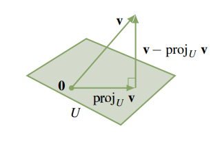
The vectors \(\mathbf{v}, \operatorname{proj}_{U} \mathbf{v}\), and \(\mathbf{v}-\operatorname{proj}_{U} \mathbf{v}\) in Theorem \(\PageIndex{7}\) can be visualized geometrically as in the diagram (where \(U\) is shaded and \(\operatorname{dim} U=2\) ). This suggests that \(\operatorname{proj}_{U} \mathbf{v}\) is the vector in \(U\) closest to \(\mathbf{v}\). This is, in fact, the case.

Theorem \(\PageIndex{8}\)

Let \(U\) be a finite dimensional subspace of an inner product space \(V\). If \(\mathbf{v}\) is any vector in \(V\), then \(\operatorname{proj}_{U} \mathbf{v}\) is the vector in \(U\) that is closest to \(\mathbf{v}\). Here closest means that

\[
\left\|\mathbf{v}-\operatorname{proj}_{U} \mathbf{v}\right\|<\|\mathbf{v}-\mathbf{u}\|
\]

for all \(\mathbf{u}\) in \(U, \mathbf{u} \neq \operatorname{proj}_{U} \mathbf{v}\).

Proof. Write \(\mathbf{p}=\operatorname{proj}_{U} \mathbf{v}\), and consider \(\mathbf{v}-\mathbf{u}=(\mathbf{v}-\mathbf{p})+(\mathbf{p}-\mathbf{u})\). Because \(\mathbf{v}-\mathbf{p}\) is in \(U^{\perp}\) and \(\mathbf{p}-\mathbf{u}\) is in \(U\), Pythagoras' theorem gives

\[
\|\mathbf{v}-\mathbf{u}\|^{2}=\|\mathbf{v}-\mathbf{p}\|^{2}+\|\mathbf{p}-\mathbf{u}\|^{2}>\|\mathbf{v}-\mathbf{p}\|^{2}
\]

because \(\mathbf{p}-\mathbf{u} \neq 0\). The result follows.

Example \(\PageIndex{6}\)

Consider the space \(\mathbf{C}[-1,1]\) of real-valued continuous functions on the interval \([-1,1]\) with inner product \(\langle f, g\rangle=\int_{-1}^{1} f(x) g(x) d x\). Find the polynomial \(p=p(x)\) of degree at most 2 that best approximates the absolute-value function \(f\) given by \(f(x)=|x|\).

Solution

Here we want the vector \(p\) in the subspace \(U=\mathbf{P}_{2}\) of \(\mathbf{C}[-1,1]\) that is closest to \(f\). In Example 10.2.4 the Gram-Schmidt algorithm was applied to give an orthogonal basis \(\left\{\mathbf{f}_{1}=1, \mathbf{f}_{2}=x, \mathbf{f}_{3}=3 x^{2}-1\right\}\) of \(\mathbf{P}_{2}\) (where, for convenience, we have changed \(\mathbf{f}_{3}\) by a numerical factor). Hence the required polynomial is

\[
\begin{aligned}
p & =\operatorname{proj}_{\mathbf{P}_{2}} f \\
& =\frac{\left\langle f, \mathbf{f}_{1}\right\rangle}{\left\|\mathbf{f}_{1}\right\|^{2}} \mathbf{f}_{1}+\frac{\left\langle f, \mathbf{f}_{2}\right\rangle}{\left\|\mathbf{f}_{2}\right\|^{2}} \mathbf{f}_{2}+\frac{\left\langle f, \mathbf{f}_{3}\right\rangle}{\left\|\mathbf{f}_{3}\right\|^{2}} \mathbf{f}_{3} \\
& =\frac{1}{2} \mathbf{f}_{1}+0 \mathbf{f}_{2}+\frac{1 / 2}{8 / 5} \mathbf{f}_{3} \\
& =\frac{3}{16}\left(5 x^{2}+1\right)
\end{aligned}
\]

Figure \(\PageIndex{2}\)

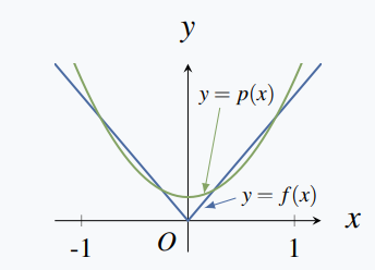
The graphs of \(p(x)\) and \(f(x)\) are given in the diagram.

If polynomials of degree at most \(n\) are allowed in Example 10.2.6, the polynomial in \(\mathbf{P}_{n}\) is \(\operatorname{proj}_{\mathbf{P}_{n}} f\), and it is calculated in the same way. Because the subspaces \(\mathbf{P}_{n}\) get larger as \(n\) increases, it turns out that the approximating polynomials \(\operatorname{proj}_{\mathbf{P}_{n}} f\) get closer and closer to \(f\). In fact, solving many practical problems comes down to approximating some interesting vector \(\mathbf{v}\) (often a function) in an infinite dimensional inner product space \(V\) by vectors in finite dimensional subspaces (which can be computed). If \(U_{1} \subseteq U_{2}\) are finite dimensional subspaces of \(V\), then

\[
\left\|\mathbf{v}-\operatorname{proj}_{U_{2}} \mathbf{v}\right\| \leq\left\|\mathbf{v}-\operatorname{proj}_{U_{1}} \mathbf{v}\right\|
\]

by Theorem 10.2.8 (because \(\operatorname{proj}_{U_{1}} \mathbf{v}\) lies in \(U_{1}\) and hence in \(U_{2}\) ). Thus \(\operatorname{proj}_{U_{2}} \mathbf{v}\) is a better approximation to \(\mathbf{v}\) than \(\operatorname{proj}_{U_{1}} \mathbf{v}\). Hence a general method in approximation theory might be described as follows: Given \(\mathbf{v}\), use it to construct a sequence of finite dimensional subspaces

\[
U_{1} \subseteq U_{2} \subseteq U_{3} \subseteq \cdots
\]

of \(V\) in such a way that \(\left\|\mathbf{v}-\operatorname{proj}_{U_{k}} \mathbf{v}\right\|\) approaches zero as \(k\) increases. Then \(\operatorname{proj}_{U_{k}} \mathbf{v}\) is a suitable approximation to \(\mathbf{v}\) if \(k\) is large enough. For more information, the interested reader may wish to consult Interpolation and Approximation by Philip J. Davis (New York: Blaisdell, 1963).