
10.12: Data Structures for Graphs
- Page ID
- 86164

\( \newcommand{\vecs}[1]{\overset { \scriptstyle \rightharpoonup} {\mathbf{#1}} } \)
\( \newcommand{\vecd}[1]{\overset{-\!-\!\rightharpoonup}{\vphantom{a}\smash {#1}}} \)
\( \newcommand{\dsum}{\displaystyle\sum\limits} \)
\( \newcommand{\dint}{\displaystyle\int\limits} \)
\( \newcommand{\dlim}{\displaystyle\lim\limits} \)
\( \newcommand{\id}{\mathrm{id}}\) \( \newcommand{\Span}{\mathrm{span}}\)
( \newcommand{\kernel}{\mathrm{null}\,}\) \( \newcommand{\range}{\mathrm{range}\,}\)
\( \newcommand{\RealPart}{\mathrm{Re}}\) \( \newcommand{\ImaginaryPart}{\mathrm{Im}}\)
\( \newcommand{\Argument}{\mathrm{Arg}}\) \( \newcommand{\norm}[1]{\| #1 \|}\)
\( \newcommand{\inner}[2]{\langle #1, #2 \rangle}\)
\( \newcommand{\Span}{\mathrm{span}}\)
\( \newcommand{\id}{\mathrm{id}}\)
\( \newcommand{\Span}{\mathrm{span}}\)
\( \newcommand{\kernel}{\mathrm{null}\,}\)
\( \newcommand{\range}{\mathrm{range}\,}\)
\( \newcommand{\RealPart}{\mathrm{Re}}\)
\( \newcommand{\ImaginaryPart}{\mathrm{Im}}\)
\( \newcommand{\Argument}{\mathrm{Arg}}\)
\( \newcommand{\norm}[1]{\| #1 \|}\)
\( \newcommand{\inner}[2]{\langle #1, #2 \rangle}\)
\( \newcommand{\Span}{\mathrm{span}}\) \( \newcommand{\AA}{\unicode[.8,0]{x212B}}\)
\( \newcommand{\vectorA}[1]{\vec{#1}} % arrow\)
\( \newcommand{\vectorAt}[1]{\vec{\text{#1}}} % arrow\)
\( \newcommand{\vectorB}[1]{\overset { \scriptstyle \rightharpoonup} {\mathbf{#1}} } \)
\( \newcommand{\vectorC}[1]{\textbf{#1}} \)
\( \newcommand{\vectorD}[1]{\overrightarrow{#1}} \)
\( \newcommand{\vectorDt}[1]{\overrightarrow{\text{#1}}} \)
\( \newcommand{\vectE}[1]{\overset{-\!-\!\rightharpoonup}{\vphantom{a}\smash{\mathbf {#1}}}} \)
\( \newcommand{\vecs}[1]{\overset { \scriptstyle \rightharpoonup} {\mathbf{#1}} } \)
\(\newcommand{\longvect}{\overrightarrow}\)
\( \newcommand{\vecd}[1]{\overset{-\!-\!\rightharpoonup}{\vphantom{a}\smash {#1}}} \)
\(\newcommand{\avec}{\mathbf a}\) \(\newcommand{\bvec}{\mathbf b}\) \(\newcommand{\cvec}{\mathbf c}\) \(\newcommand{\dvec}{\mathbf d}\) \(\newcommand{\dtil}{\widetilde{\mathbf d}}\) \(\newcommand{\evec}{\mathbf e}\) \(\newcommand{\fvec}{\mathbf f}\) \(\newcommand{\nvec}{\mathbf n}\) \(\newcommand{\pvec}{\mathbf p}\) \(\newcommand{\qvec}{\mathbf q}\) \(\newcommand{\svec}{\mathbf s}\) \(\newcommand{\tvec}{\mathbf t}\) \(\newcommand{\uvec}{\mathbf u}\) \(\newcommand{\vvec}{\mathbf v}\) \(\newcommand{\wvec}{\mathbf w}\) \(\newcommand{\xvec}{\mathbf x}\) \(\newcommand{\yvec}{\mathbf y}\) \(\newcommand{\zvec}{\mathbf z}\) \(\newcommand{\rvec}{\mathbf r}\) \(\newcommand{\mvec}{\mathbf m}\) \(\newcommand{\zerovec}{\mathbf 0}\) \(\newcommand{\onevec}{\mathbf 1}\) \(\newcommand{\real}{\mathbb R}\) \(\newcommand{\twovec}[2]{\left[\begin{array}{r}#1 \\ #2 \end{array}\right]}\) \(\newcommand{\ctwovec}[2]{\left[\begin{array}{c}#1 \\ #2 \end{array}\right]}\) \(\newcommand{\threevec}[3]{\left[\begin{array}{r}#1 \\ #2 \\ #3 \end{array}\right]}\) \(\newcommand{\cthreevec}[3]{\left[\begin{array}{c}#1 \\ #2 \\ #3 \end{array}\right]}\) \(\newcommand{\fourvec}[4]{\left[\begin{array}{r}#1 \\ #2 \\ #3 \\ #4 \end{array}\right]}\) \(\newcommand{\cfourvec}[4]{\left[\begin{array}{c}#1 \\ #2 \\ #3 \\ #4 \end{array}\right]}\) \(\newcommand{\fivevec}[5]{\left[\begin{array}{r}#1 \\ #2 \\ #3 \\ #4 \\ #5 \\ \end{array}\right]}\) \(\newcommand{\cfivevec}[5]{\left[\begin{array}{c}#1 \\ #2 \\ #3 \\ #4 \\ #5 \\ \end{array}\right]}\) \(\newcommand{\mattwo}[4]{\left[\begin{array}{rr}#1 \amp #2 \\ #3 \amp #4 \\ \end{array}\right]}\) \(\newcommand{\laspan}[1]{\text{Span}\{#1\}}\) \(\newcommand{\bcal}{\cal B}\) \(\newcommand{\ccal}{\cal C}\) \(\newcommand{\scal}{\cal S}\) \(\newcommand{\wcal}{\cal W}\) \(\newcommand{\ecal}{\cal E}\) \(\newcommand{\coords}[2]{\left\{#1\right\}_{#2}}\) \(\newcommand{\gray}[1]{\color{gray}{#1}}\) \(\newcommand{\lgray}[1]{\color{lightgray}{#1}}\) \(\newcommand{\rank}{\operatorname{rank}}\) \(\newcommand{\row}{\text{Row}}\) \(\newcommand{\col}{\text{Col}}\) \(\renewcommand{\row}{\text{Row}}\) \(\newcommand{\nul}{\text{Nul}}\) \(\newcommand{\var}{\text{Var}}\) \(\newcommand{\corr}{\text{corr}}\) \(\newcommand{\len}[1]{\left|#1\right|}\) \(\newcommand{\bbar}{\overline{\bvec}}\) \(\newcommand{\bhat}{\widehat{\bvec}}\) \(\newcommand{\bperp}{\bvec^\perp}\) \(\newcommand{\xhat}{\widehat{\xvec}}\) \(\newcommand{\vhat}{\widehat{\vvec}}\) \(\newcommand{\uhat}{\widehat{\uvec}}\) \(\newcommand{\what}{\widehat{\wvec}}\) \(\newcommand{\Sighat}{\widehat{\Sigma}}\) \(\newcommand{\lt}{<}\) \(\newcommand{\gt}{>}\) \(\newcommand{\amp}{&}\) \(\definecolor{fillinmathshade}{gray}{0.9}\)In this section, we will describe data structures that are commonly used to represent graphs. In addition we will introduce the basic syntax for graphs in Sage.
Basic Data Structures
List \(\PageIndex{1}\): Data Structures for Graphs
Assume that we have a graph with \(n\) vertices that can be indexed by the integers \(1, 2, \dots, n\text{.}\) Here are three different data structures that can be employed to represent graphs.
- Adjacency Matrix: As we saw in Chapter 6, the information about edges in a graph can be summarized with an adjacency matrix, \(G\text{,}\) where \(G_{ij}=1\) if and only if vertex \(i\) is connected to vertex \(j\) in the graph. Note that this is the same as the adjacency matrix for a relation.
- Edge Dictionary: For each vertex in our graph, we maintain a list of edges that initiate at that vertex. If \(G\) represents the graph's edge information, then we denote by \(G_i\) the list of vertices that are terminal vertices of edges initiating at vertex \(i\text{.}\) The exact syntax that would be used can vary. We will use Sage/Python syntax in our examples.
- Edge List: Note that in creating either of the first two data structures, we would presume that a list of edges for the graph exists. A simple way to represent the edges is to maintain this list of ordered pairs, or two element sets, depending on whether the graph is intended to be directed or undirected. We will not work with this data structure here, other than in the first example.
Example \(\PageIndex{1}\): A Very Small Example
We consider the representation of the following graph:
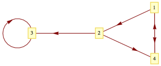 Figure \(\PageIndex{1}\): Graph for a Very Small Example
The adjacency matrix that represents the graph would be
\begin{equation*} G=\left( \begin{array}{cccc} 0 & 1 & 0 & 1 \\ 0 & 0 & 1 & 1 \\ 0 & 0 & 1 & 0 \\ 1 & 0 & 0 & 0 \\ \end{array} \right)\text{.} \end{equation*}
The same graph could be represented with the edge dictionary
{1:[2,4],2:[3,4],3:[3],4:[1]}.
Notice the general form of each item in the dictionary: vertex:[list of vertices].
Finally, a list of edges [(1,2),(1,4),(2,3),(2,4),(3,3),(4,1)] also describes the same graph.
A natural question to ask is: Which data structure should be used in a given situation? For small graphs, it really doesn't make much difference. For larger matrices the edge count would be a consideration. If \(n\) is large and the number of edges is relatively small, it might use less memory to maintain an edge dictionary or list of edges instead of building an \(n \times n\) matrix. Some software for working with graphs will make the decision for you.
Example \(\PageIndex{2}\): NCAA Basketball
Consider the tournament graph representing a NCAA Division 1 men's (or women's) college basketball season in the United States. There are approximately 350 teams in Division 1. Suppose we constructed the graph with an edge from team A to team B if A beat B at least once in the season; and we label the edge with the number of wins. Since the average team plays around 30 games in a season, most of which will be against other Division I teams, we could expect around \(\frac{30 \cdot 350}{2}=5,250\) edges in the graph. This would be somewhat reduced by games with lower division teams and cases where two or more wins over the same team produces one edge. Since 5,250 is much smaller than \(350^2=122,500\) entries in an adjacency matrix, an edge dictionary or edge list would be more compact than an adjacency matrix. Even if we were to use software to create an adjacency matrix, many programs will identify the fact that a matrix such as the one in this example would be “sparse” and would leave data in list form and use sparse array methods to work with it.
Graphs
The most common way to define a graph in Sage is to use an edge dictionary. Here is how the graph in Example \(\PageIndex{1}\) is generated and then displayed. Notice that we simply wrap the function DiGraph() around the same dictionary expression we identified earlier.
G1 = DiGraph( {1 : [4, 2], 2 : [3, 4], 3 : [3], 4 : [1]})
G1.show()
You can get the adjacency matrix of a graph with the adjacency_matrix method.
G1.adjacency_matrix()
You can also define a graph based on its adjacency matrix.
M = Matrix([[0,1,0,0,0],[0,0,1,0,0],[0,0,0,1,0],
              [0,0,0,0,1],[1,0,0,0,0]])
DiGraph(M).show()
The edge list of any directed graph can be easily retrieved. If you replace edges with edge_iterator, you can iterate through the edge list. The third coordinate of the items in the edge is the label of the edge, which is None in this case.
DiGraph(M).edges()
Replacing the wrapper DiGraph() with Graph() creates an undirected graph.
G2 = Graph( {1 : [4, 2], 2 : [3, 4], 3 : [3], 4 : [1]})
G2.show()
There are many special graphs and graph families that are available in Sage through the graphs module. They are referenced with the prefix graphs. followed by the name and zero or more parameters inside parentheses. Here are a couple of them, first a complete graph with five vertices.
graphs.CompleteGraph(5).show()
Here is a wheel graph, named for an obvious pattern of vertices and edges. We assign a name to it first and then show the graph without labeling the vertices.
w=graphs.WheelGraph(20)
w.show(vertex_labels=false)
There are dozens of graph methods, one of which determines the degree sequence of a graph. In this case, it's the wheel graph above.
w.degree_sequence()
The degree sequence method is defined within the graphs module, but the prefix graphs. is not needed because the value of w inherits the graphs methods.
Exercises
Exercise \(\PageIndex{1}\)
Estimate the number of vertices and edges in each of the following graphs. Would the graph be considered sparse, so that an adjacency matrix would be inefficient?
- Vertices: Cities of the world that are served by at least one airline. Edges: Pairs of cities that are connected by a regular direct flight.
- Vertices: ASCII characters. Edges: connect characters that differ in their binary code by exactly two bits.
- Vertices: All English words. Edges: An edge connects word \(x\) to word \(y\) if \(x\) is a prefix of \(y\text{.}\)
- Answer
-
- A rough estimate of the number of vertices in the “world airline graph” would be the number of cities with population greater than or equal to 100,000. This is estimated to be around 4,100. There are many smaller cities that have airports, but some of the metropolitan areas with clusters of large cities are served by only a few airports. 4,000-5,000 is probably a good guess. As for edges, that's a bit more difficult to estimate. It's certainly not a complete graph. Looking at some medium sized airports such as Manchester, NH, the average number of cities that you can go to directly is in the 50-100 range. So a very rough estimate would be \(\frac{75 \cdot 4500}{2}=168,750\text{.}\) This is far less than \(4,500^2\text{,}\) so an edge list or dictionary of some kind would be more efficient.
- The number of ASCII characters is 128. Each character would be connected to \(\binom{8}{2}=28\) others and so there are \(\frac{128 \cdot 28}{2}=3,584\) edges. Comparing this to the \(128^2=16,384\text{,}\) an array is probably the best choice.
- The Oxford English Dictionary as approximately a half-million words, although many are obsolete. The number of edges is probably of the same order of magnitude as the number of words, so an edge list or dictionary is probably the best choice.
Exercise \(\PageIndex{2}\)
Each edge of a graph is colored with one of the four colors red, blue, yellow, or green. How could you represent the edges in this graph using a variation of the adjacency matrix structure?
Exercise \(\PageIndex{3}\)
Directed graphs \(G_1, \dots, G_6\) , each with vertex set \(\{1,2,3,4,5\}\) are represented by the matrices below. Which graphs are isomorphic to one another?
\(G_1: \left( \begin{array}{ccccc} 0 & 1 & 0 & 0 & 0 \\ 0 & 0 & 1 & 0 & 0 \\ 0 & 0 & 0 & 1 & 0 \\ 0 & 0 & 0 & 0 & 1 \\ 1 & 0 & 0 & 0 & 0 \\ \end{array} \right)\)\(\quad \quad\)\(G_2: \left( \begin{array}{ccccc} 0 & 0 & 0 & 0 & 0 \\ 0 & 0 & 1 & 0 & 0 \\ 0 & 0 & 0 & 0 & 0 \\ 1 & 1 & 1 & 0 & 1 \\ 0 & 0 & 0 & 0 & 0 \\ \end{array} \right)\)\(\quad \quad\)\(G_3: \left( \begin{array}{ccccc} 0 & 0 & 0 & 0 & 0 \\ 1 & 0 & 0 & 0 & 1 \\ 0 & 1 & 0 & 0 & 0 \\ 0 & 0 & 1 & 0 & 0 \\ 0 & 0 & 1 & 0 & 0 \\ \end{array} \right)\) \(G_4: \left( \begin{array}{ccccc} 0 & 1 & 1 & 1 & 1 \\ 0 & 0 & 0 & 0 & 0 \\ 0 & 0 & 0 & 0 & 0 \\ 0 & 0 & 1 & 0 & 0 \\ 0 & 0 & 0 & 0 & 0 \\ \end{array} \right)\)\(\quad \quad\)\(\quad G_5: \left( \begin{array}{ccccc} 0 & 0 & 0 & 0 & 1 \\ 0 & 0 & 0 & 0 & 0 \\ 0 & 1 & 0 & 1 & 0 \\ 0 & 0 & 0 & 0 & 1 \\ 0 & 0 & 1 & 0 & 0 \\ \end{array} \right)\)\(\quad \quad\)\(G_6: \left( \begin{array}{ccccc} 0 & 0 & 0 & 1 & 0 \\ 0 & 0 & 0 & 0 & 0 \\ 1 & 1 & 0 & 0 & 0 \\ 0 & 0 & 1 & 0 & 0 \\ 0 & 0 & 0 & 1 & 0 \\ \end{array} \right)\)
- Answer
-
Each graph is isomorphic to itself. In addition, \(G_2 \text{ and } G_4\) are isomorphic; and \(G_3, G_5, \text{ and } G_6\) are isomorphic to one another.
Exercise \(\PageIndex{4}\)
The following Sage command verifies that the wheel graph with four vertices is isomorphic to the complete graph with four vertices.
graphs.WheelGraph(4).is_isomorphic(graphs.CompleteGraph(4))
A list of all graphs in this the graphs database is available via tab completion. Type "graphs." and then hit the tab key to see which graphs are available. This can be done using the Sage application or SageMathCloud, but not sage cells. Find some other pairs of isomorphic graphs in the database.