5.5 Chapter 5 Study Guide

Definitions

• (Recall) linear function: a degree-1 polynomial function of the form \( f(x) = a_1 x + a_0 \), aka \( f(x) = mx + b\).
• average rate of change: the rate of change of \(y=f(x)\) with respect to \(x\) between \(x = a\) and \( x = b\) is \( \dfrac{ f(b)-f(a)}{b-a} \), aka like slope of a straight line between two data points \( (a,f(a)), (b,f(b)) \).
• secant line: a straight line drawn between two points on the graph of a function, \( (a,f(a)) \) and \( (b,f(b))\).
• quadratic function: a degree-2 polynomial function of the form \( f(x) = a_2 x^2 + a_1 x + a_0 \), aka \( f(x) = ax^2 + bx + c\).
• vertex form: the equation of a parabola in the form \( f(x) = a(x-h)^2 +k\), highlighting the location of the vertex \( (h,k) \).
• polynomial function: a function that can be written in the form \( f(x) = a_n x^n + a_{n-1}x^{n-1} + \cdots + a_1 x + a_0 \).
• roots / zeros: the roots \(x = c \) of a polynomial function are the locations of the \(x\)-intercepts, found by setting the function equal to 0 and solving for \(x\).
• multiplicity: the multiplicity of a root \(x = c\) is the number of copies of \( (x-c)\) that appear in the polynomial's factorization.
• linear factors: factors of the form \( (x-c)\).
• irreducible quadratic factors: factors of the form \( (ax^2 + bx + c)\) that do not yield real roots, aka the discriminant \(b^2 - 4ac < 0\).
• polynomial long division: the process of dividing a polynomial \(p(x)\) by a divisor polynomial \(d(x)\), resulting in a quotient polynomial \(q(x)\) and potentially a remainder \(r(x)\). Results are written in the forms
  \[ \frac{ p(x)}{d(x)} = q(x) + \frac{ r(x)}{d(x)} \quad \text{ and } \quad p(x) = q(x) \cdot d(x) + r(x) \notag \]
• end behavior: how a function behaves as you look off in the positive or negative \(x\)-direction forever, written like "as \(x\rightarrow \infty\), \(f(x) \rightarrow \infty\)" for example.

Facts About Linear Functions

• Both the domain and the range of a linear function (unless specified due to an application) are all real numbers, \( \mathbb{R}\).
• The graphs of linear functions are straight lines. If you rename \(a_1 = m\) and \(a_0 = b\), you can recognize the slope-intercept equation of a line.
• Consequently, the leading coefficient \(a_1\) gives the slope of the line, and the constant term \(a_0\) gives the \(y\)-intercept \( (0, a_0) \) of the graph.
• Because of what we know about positive and negative slopes, if \(a_1 < 0 \), the function is decreasing (going downhill from left to right) and if \( a_1 > 0 \), the function is increasing (going uphill from left to right).
• Linear functions have constant rate of change (slope is the same no matter what two points are used to calculate it). You can check if a table of values defines a linear function by checking if all slope calculations between data points give the same result.

Facts About Quadratic Functions

• The graphs of these functions are parabolas, which can open upward or downward. If the leading coefficient \(a > 0\), it opens upward. If \(a < 0\), it opens downward. There is a point called the vertex, which is the peak of the hill if the parabola opens downward, or the bottom of the trough if the parabola opens upward. The parabola is symmetric about the vertical line passing through the vertex.
• Quadratics are often written in vertex form, \( f(x) = a(x-h)^2 + k\), highlighting the location of the parabola's vertex, \( (h,k)\). ALERT: be careful with the signs because of that subtraction!
• The domain of a quadratic function (unless specified due to an application) is all real numbers, \(\mathbb{R}\).
• The range of a quadratic function is limited due to its parabola shape. Identifying the vertex will help you determine the range, since it will give the maximum or minimum possible function value.
• The \(x\)-intercept(s) of quadratic functions are called roots or zeros. As always, to find these, set the whole function equal to 0 and solve for \(x\).
  • A quadratic can have (a) one repeated real root, (b) two distinct real roots, or (c) no real roots (but rather a complex conjugate pair of roots).
  • In case (a), the parabola bounces off the \(x\)-axis. In case (b), the parabola intersects the \(x\)-axis at two locations. In case (c), the parabola is too low or too high and never intersects the \(x\)-axis.

Converting From Standard Form to Vertex Form

To convert from standard form \(f(x) = ax^2 + bx + c \) into vertex form \( f(x) = a(x-h)^2 + k \),

1. If \(a \neq 1\), factor it out like so: \( f(x) = a \left( x^2 + \frac{b}{a} x + \frac{c}{a} \right) \).
2. Working inside the parentheses, complete the square on the first two terms, \(x^2 + \frac{b}{a} x \), making sure to both add and subtract the necessary term inside the parentheses.
3. If necessary, distribute the factored-out \(a\) back onto the constant term to finally reach the form \( f(x) = a(x-h)^2 + k \) for some \(h\) and \(k\).

Sketching Quadratic Functions

1. Find the vertex form and plot the vertex. Note whether the parabola should open up or down.
2. Find a few more points by plugging in different \(x\)-values and computing the function values. You can also choose to find the roots instead of random points.
3. Using knowledge of symmetry and how parabolas look, fit a parabola to the the plotted points smoothly.

Or, use knowledge of transformations to sketch the graph, starting with the most basic \( f(x) = x^2\) and performing the appropriate transformations.

Facts About Polynomial Functions

• The highest appearing power \(n\) is called the degree.
• These functions always have all real numbers as their domain.
• The range of a polynomial function depends on whether its degree is even or odd and the sign of its leading coefficient. We'll talk about this and end behavior later.
• The \(x\)-intercepts are called the roots or zeros of the polynomial function. The maximum number of real roots for a given degree-\(n\) polynomial, counting with multiplicity, is \(n\).
• The graphs of polynomials are always nicely smoothly curved, with no skips or jumps or corners.

Table of Polynomial Examples

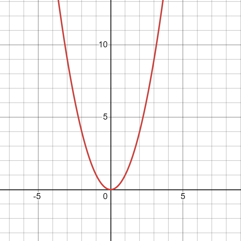
degree 2 (quadratic)	degree 3 (cubic)	degree 4 (quartic)	degree 5
\( f(x) = x^2 \)	\( f(x) = x^3 \)	\( f(x) = x^4 \)	\( f(x) = x^5 \)
\( f(x) =(x-3)(x+2) \)	\( f(x) = (x-1)(x+1)(x-2) \)	\( f(x) = x(x-2)(x-1)(x+2)\)	\( f(x) = x(x-2)(x-2)(x+1)(x+2) \)
\( f(x) = -(x-1)^2 \)	\( f(x) = -(x-2)^2(x+1) \)	\( f(x) = -(x+1)^2(x-1)^2 \)	\( f(x) = -x(x-2)^4 \)
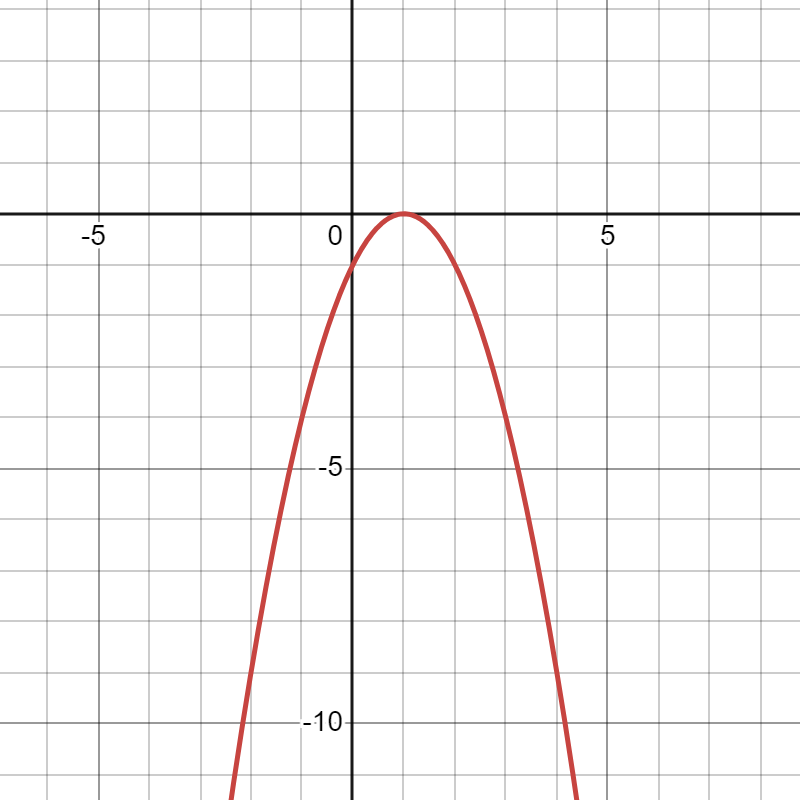
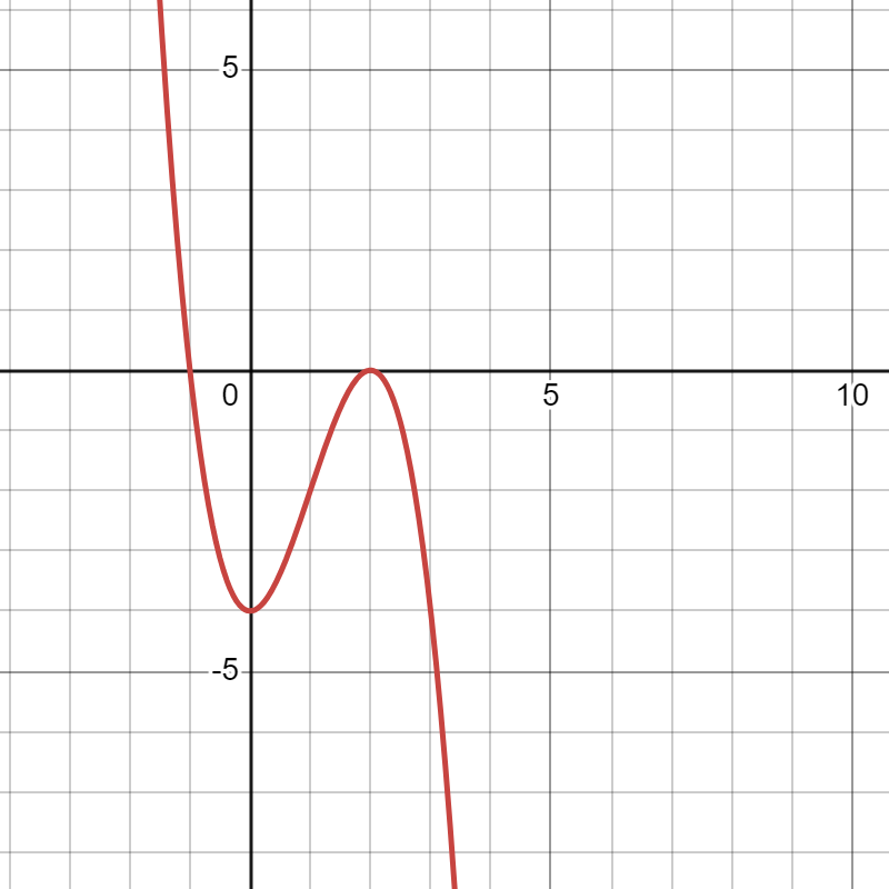
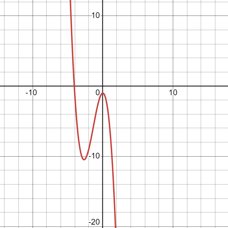
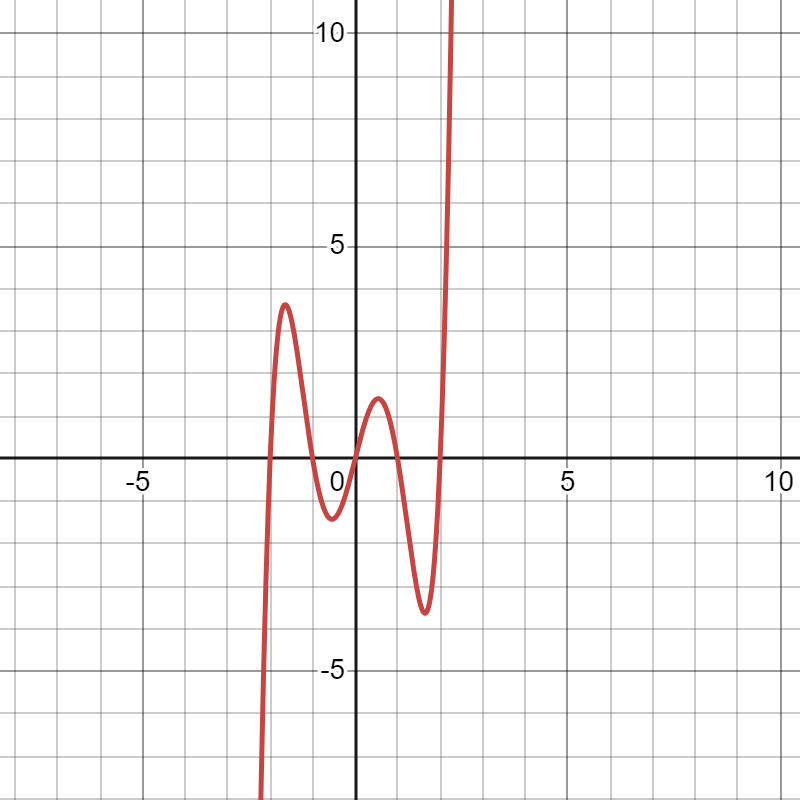
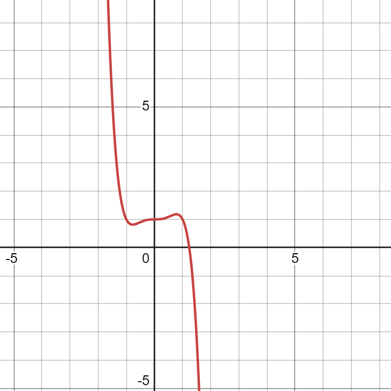
\( f(x) = -x^2 + 3x - 3 \)	\( f(x) = -x^3 - 4x^2 - 1 \)	\( f(x) = x^4 - x^2 - x + 2 \)	\( f(x) = -x^5 + x^3 + 1 \)

Notes:

• Monomials like \(f(x) = x^n\) for even power \(n\) kind of look like parabolas but flattening out more at the origin. If \(n\) is odd, they look like the basic cubic, but flattening out more at the origin.
• A degree-\(n\) polynomial function can "turn around" (have a peak or a trough) up to \(n-1\) times. For example, the degree-four polynomials can't have more than three turnarounds.
• A degree-\(n\) polynomial function can have up to \(n\) distinct real roots.
• End behavior: see table summarizing below.

End Behavior

degree vs. sign of leading coefficient	\( a_n > 0 \)	\( a_n < 0 \)
\( n\) even	as \(x \rightarrow \infty\), \(f(x) \rightarrow \infty\) as \(x \rightarrow -\infty\), \(f(x) \rightarrow \infty\)	as \(x \rightarrow \infty\), \(f(x) \rightarrow -\infty\) as \(x \rightarrow -\infty\), \(f(x) \rightarrow -\infty\)
\( n\) odd	as \(x \rightarrow \infty\), \(f(x) \rightarrow \infty\) as \(x \rightarrow -\infty\), \(f(x) \rightarrow -\infty\)	as \(x \rightarrow \infty\), \(f(x) \rightarrow -\infty\) as \(x \rightarrow -\infty\), \(f(x) \rightarrow \infty\)

Roots and Multiplicity

The real number \( c\) is a root (zero) of a polynomial function \( p(x) \) if and only (iff) the factor \( (x-c)\) appears in the factorization of \( p(x) \). The multiplicity of the root \(c\) is the number of times that factor is repeated in the factorization. So if

\[ p(x) = (\: \cdots \: ) \cdots (x-c)^n \cdots (\: \cdots\: ) \notag \]

then the multiplicity of root \(c\) is \(n\).

Multiplicity and graphs:

• When a root has multiplicity 1, the graph passes straight through the \(x\)-axis at that point.
• When a root has multiplicity 2, the graph bounces off the \(x\)-axis at that point.
• When a root has multiplicity 3, the graph passes through the \(x\)-axis, but it hangs out for a second, flattening out a bit.
• When a root has multiplicity 4, the graph bounces off the \(x\)-axis, but it hangs out for a second, flattening out a bit.
• The pattern continues: pass through the \(x\)-axis at odd multiplicity roots, but don't cross over at even multiplicity roots, and the higher the multiplicity, the more flattening behavior.

Polynomial Long Division

1. Insert placeholders with zero coefficients for any missing powers of \(x\) in the dividend \(p(x)\). Set up long division bar with \( p(x)\) underneath and \(d(x)\) out front.
2. Compare first terms to see what is missing. Write whatever factors are needed to make them match up above the division bar in the appropriate column.
3. Perform the multiplication through \(d(x)\), writing it underneath \(p(x)\) in appropriate columns. Subtract down the columns. Bring down next term.
4. Compare the first terms, repeat Steps 2-3 until no more terms to bring down.
5. Terms written above the bar are \(q(x)\), and remainder is \(r(x)\).

Example

Divide \(p(x) = x^4 - 1\) by \( d(x) = x^2 - 1\). Write the result in the form \( p(x) = q(x) \cdot d(x) + r(x) \), and in the form \(\frac{ p(x)}{d(x)} = q(x) + \frac{ r(x)}{d(x)}\).

Solution

First, I insert placeholders: \( p(x) = x^4 + 0x^3 + 0x^2 + 0x - 1\). I write this below the long division sign and put \(d(x)\) out front.

\begin{array}{r}
\phantom{)} \\
x^2-1{\overline{\smash{\big)}\,x^4 + 0x^3 + 0x^2 + 0x - 1\phantom{)}}}\\
\notag
\end{array}

Comparing the first terms, I need to multiply \(x^2\) by \(x^2\) to make it match the \(x^4\) so that they will kill each other off when I subtract. Place that up above, and perform the multiplication, writing it underneath in the appropriate columns. Subtract down the columns and bring down the next term(s).

\begin{array}{r}
x^2\phantom{+0x^2+1}\phantom{)} \\
x^2-1{\overline{\smash{\big)}\,x^4 + 0x^3 + 0x^2 + 0x - 1\phantom{)}}}\\
\underline{-~\phantom{(}(x^4\qquad \quad -x^2)\phantom{ + 0x - 1b)}}\\
0+0+x^2 \textcolor{red}{+0x-1}\phantom{)}\\
\notag
\end{array}

Now we compare the first terms and see that \(x^2\) already matches \(x^2\). When this happens, you don't need to multiply by anything but 1, so put a 1 above the division bar. We perform the multiplication and write it underneath, lined up correctly. Subtract again.

\begin{array}{r}
x^2 \quad \quad+1\phantom{)} \\
x^2-1{\overline{\smash{\big)}\,x^4 + 0x^3 + 0x^2 + 0x - 1\phantom{)}}}\\
\underline{-~\phantom{(}(x^4\qquad \quad -x^2)\phantom{ + 0x - 1b)}}\\
0+0+x^2 +0x-1\phantom{)}\\
\underline{-~\phantom{()}(x^2 \quad \quad -1)}\\
0\phantom{)}
\notag
\end{array}

Notice that on our last subtraction, everything wiped out, leaving a remainder of \( r(x) = 0\)! This means that the divisor \(d(x)\) divides evenly into \(p(x)\). We write our final answer:

\[ x^4 - 1 = (x^2 +1)(x^2 -1) \quad \text{ or } \quad \frac{x^4 - 1}{x^2-1} = x^2+1 \notag \]

Rational Root Theorem

If a polynomial \( f(x) = a_n x^n + a_{n-1}x^{n-1} + \cdots + a_1 x + a_0 \) has integer coefficients \(a_n \neq 0\) and \( a_0 \neq 0\), then every rational root of \(f\) is of the form \( \dfrac{p}{q} \), where \(p\) is a factor of \(a_0\), and \(q\) is a factor of \(a_n\).

In other words, to find the list of possible rational number roots of \(f\), make two lists,

• all the integer factors \(\pm p_1, \pm p_2, \pm p_3 ... \) of the constant term \(a_0\),
• all the integer factors \(\pm q_1, \pm q_2, \pm q_3 ... \) of the leading coefficient \(a_n\),

and then list all possible combinations \(\pm \dfrac{p_i}{q_j}\) where the numerator is from the first list and the denominator is from the second list. These are the only rational numbers that could be roots of \(f\), and you can check which are actually roots by evaluating \(f\) to see if you get zero there.

Factoring Higher-Degree Polynomial Functions

To factor a polynomial function \(f\) and find its real roots:

Step 1: Find a root \(c\) by inspection. One you find \(c\), you know \( (x-c)\) must appear in the polynomial's factorization, like \( f(x) = (x-c)( \text{something else}) \).

Step 2: Divide \(f\) by \( (x-c)\) using polynomial division. The quotient \(q(x)\) is the \( (\text{something else})\) factor.

Step 3: If the \(q(x)\) is not a linear factor or an irreducible quadratic, repeat the process on \(q(x)\) to further factor it. So on and so forth, until every factor is linear of the form \( (x-c)\) or an irreducible quadratic.

Step 4: Determine the real roots using the linear factors.