
6.1 Rational Functions
- Page ID
- 155158

\( \newcommand{\vecs}[1]{\overset { \scriptstyle \rightharpoonup} {\mathbf{#1}} } \)
\( \newcommand{\vecd}[1]{\overset{-\!-\!\rightharpoonup}{\vphantom{a}\smash {#1}}} \)
\( \newcommand{\dsum}{\displaystyle\sum\limits} \)
\( \newcommand{\dint}{\displaystyle\int\limits} \)
\( \newcommand{\dlim}{\displaystyle\lim\limits} \)
\( \newcommand{\id}{\mathrm{id}}\) \( \newcommand{\Span}{\mathrm{span}}\)
( \newcommand{\kernel}{\mathrm{null}\,}\) \( \newcommand{\range}{\mathrm{range}\,}\)
\( \newcommand{\RealPart}{\mathrm{Re}}\) \( \newcommand{\ImaginaryPart}{\mathrm{Im}}\)
\( \newcommand{\Argument}{\mathrm{Arg}}\) \( \newcommand{\norm}[1]{\| #1 \|}\)
\( \newcommand{\inner}[2]{\langle #1, #2 \rangle}\)
\( \newcommand{\Span}{\mathrm{span}}\)
\( \newcommand{\id}{\mathrm{id}}\)
\( \newcommand{\Span}{\mathrm{span}}\)
\( \newcommand{\kernel}{\mathrm{null}\,}\)
\( \newcommand{\range}{\mathrm{range}\,}\)
\( \newcommand{\RealPart}{\mathrm{Re}}\)
\( \newcommand{\ImaginaryPart}{\mathrm{Im}}\)
\( \newcommand{\Argument}{\mathrm{Arg}}\)
\( \newcommand{\norm}[1]{\| #1 \|}\)
\( \newcommand{\inner}[2]{\langle #1, #2 \rangle}\)
\( \newcommand{\Span}{\mathrm{span}}\) \( \newcommand{\AA}{\unicode[.8,0]{x212B}}\)
\( \newcommand{\vectorA}[1]{\vec{#1}} % arrow\)
\( \newcommand{\vectorAt}[1]{\vec{\text{#1}}} % arrow\)
\( \newcommand{\vectorB}[1]{\overset { \scriptstyle \rightharpoonup} {\mathbf{#1}} } \)
\( \newcommand{\vectorC}[1]{\textbf{#1}} \)
\( \newcommand{\vectorD}[1]{\overrightarrow{#1}} \)
\( \newcommand{\vectorDt}[1]{\overrightarrow{\text{#1}}} \)
\( \newcommand{\vectE}[1]{\overset{-\!-\!\rightharpoonup}{\vphantom{a}\smash{\mathbf {#1}}}} \)
\( \newcommand{\vecs}[1]{\overset { \scriptstyle \rightharpoonup} {\mathbf{#1}} } \)
\(\newcommand{\longvect}{\overrightarrow}\)
\( \newcommand{\vecd}[1]{\overset{-\!-\!\rightharpoonup}{\vphantom{a}\smash {#1}}} \)
\(\newcommand{\avec}{\mathbf a}\) \(\newcommand{\bvec}{\mathbf b}\) \(\newcommand{\cvec}{\mathbf c}\) \(\newcommand{\dvec}{\mathbf d}\) \(\newcommand{\dtil}{\widetilde{\mathbf d}}\) \(\newcommand{\evec}{\mathbf e}\) \(\newcommand{\fvec}{\mathbf f}\) \(\newcommand{\nvec}{\mathbf n}\) \(\newcommand{\pvec}{\mathbf p}\) \(\newcommand{\qvec}{\mathbf q}\) \(\newcommand{\svec}{\mathbf s}\) \(\newcommand{\tvec}{\mathbf t}\) \(\newcommand{\uvec}{\mathbf u}\) \(\newcommand{\vvec}{\mathbf v}\) \(\newcommand{\wvec}{\mathbf w}\) \(\newcommand{\xvec}{\mathbf x}\) \(\newcommand{\yvec}{\mathbf y}\) \(\newcommand{\zvec}{\mathbf z}\) \(\newcommand{\rvec}{\mathbf r}\) \(\newcommand{\mvec}{\mathbf m}\) \(\newcommand{\zerovec}{\mathbf 0}\) \(\newcommand{\onevec}{\mathbf 1}\) \(\newcommand{\real}{\mathbb R}\) \(\newcommand{\twovec}[2]{\left[\begin{array}{r}#1 \\ #2 \end{array}\right]}\) \(\newcommand{\ctwovec}[2]{\left[\begin{array}{c}#1 \\ #2 \end{array}\right]}\) \(\newcommand{\threevec}[3]{\left[\begin{array}{r}#1 \\ #2 \\ #3 \end{array}\right]}\) \(\newcommand{\cthreevec}[3]{\left[\begin{array}{c}#1 \\ #2 \\ #3 \end{array}\right]}\) \(\newcommand{\fourvec}[4]{\left[\begin{array}{r}#1 \\ #2 \\ #3 \\ #4 \end{array}\right]}\) \(\newcommand{\cfourvec}[4]{\left[\begin{array}{c}#1 \\ #2 \\ #3 \\ #4 \end{array}\right]}\) \(\newcommand{\fivevec}[5]{\left[\begin{array}{r}#1 \\ #2 \\ #3 \\ #4 \\ #5 \\ \end{array}\right]}\) \(\newcommand{\cfivevec}[5]{\left[\begin{array}{c}#1 \\ #2 \\ #3 \\ #4 \\ #5 \\ \end{array}\right]}\) \(\newcommand{\mattwo}[4]{\left[\begin{array}{rr}#1 \amp #2 \\ #3 \amp #4 \\ \end{array}\right]}\) \(\newcommand{\laspan}[1]{\text{Span}\{#1\}}\) \(\newcommand{\bcal}{\cal B}\) \(\newcommand{\ccal}{\cal C}\) \(\newcommand{\scal}{\cal S}\) \(\newcommand{\wcal}{\cal W}\) \(\newcommand{\ecal}{\cal E}\) \(\newcommand{\coords}[2]{\left\{#1\right\}_{#2}}\) \(\newcommand{\gray}[1]{\color{gray}{#1}}\) \(\newcommand{\lgray}[1]{\color{lightgray}{#1}}\) \(\newcommand{\rank}{\operatorname{rank}}\) \(\newcommand{\row}{\text{Row}}\) \(\newcommand{\col}{\text{Col}}\) \(\renewcommand{\row}{\text{Row}}\) \(\newcommand{\nul}{\text{Nul}}\) \(\newcommand{\var}{\text{Var}}\) \(\newcommand{\corr}{\text{corr}}\) \(\newcommand{\len}[1]{\left|#1\right|}\) \(\newcommand{\bbar}{\overline{\bvec}}\) \(\newcommand{\bhat}{\widehat{\bvec}}\) \(\newcommand{\bperp}{\bvec^\perp}\) \(\newcommand{\xhat}{\widehat{\xvec}}\) \(\newcommand{\vhat}{\widehat{\vvec}}\) \(\newcommand{\uhat}{\widehat{\uvec}}\) \(\newcommand{\what}{\widehat{\wvec}}\) \(\newcommand{\Sighat}{\widehat{\Sigma}}\) \(\newcommand{\lt}{<}\) \(\newcommand{\gt}{>}\) \(\newcommand{\amp}{&}\) \(\definecolor{fillinmathshade}{gray}{0.9}\)By the end of this section, you will be able to:
- identify rational functions and their important features: domain, roots, asymptotes, holes
- manipulate rational functions using polynomial long division and the important tool Partial Fraction Decomposition
- solve rational and polynomial inequalities
Just as a rational number is a ratio of two integers, a rational function is a ratio of two polynomials. That's all there is to it! Stuff like this:
\[ f(x) = \frac{1}{x}, \quad \quad g(x) = \frac{ x^2 + x + 1}{x - 3}, \quad \quad h(x) = \frac{x+2}{x^5 + 4x^2 + 1} \notag \]
A rational function is a function of the form
\[ r(x) = \dfrac{ p(x)}{q(x)} \notag \]
where \(p(x)\) and \(q(x)\) are polynomials. (Assume that the fraction is fully reduced; i.e. \(p\) and \(q\) have no factors in common.) Fun facts about rational functions:
- Their domain is all real numbers except any values of \(x\) that cause \(q(x)\) to be zero. You can write this in set notation as \( \{ x \: | \: q(x) \neq 0 \} \).
- Their graphs tend to be kinda complicated, with vertical lines they aren't allowed to cross (vertical asymptotes), horizontal lines they hug as they go off to the right or left (horizontal asymptotes), and sometimes slant asymptotes, diagonal straight lines that they hug instead (see the next section for more). See a note at the end of this section to learn about holes.
The most basic example is the function \(f(x) = \dfrac{1}{x} \). It has a very simple constant function \(p(x) = 1\) as numerator and very simple linear function \( q(x) = x\) as denominator. You should know what this guy in particular looks like:

If you forget, you can always plot a handful of points like I did above to reminder yourself of his shape. Notice that \(x = 0\) is not allowed in the domain of \(f\), because that would cause me to divide by zero. Looking at the graph, you can see that the function is defined for \(x\)-values getting close to 0, but not at \(x = 0\). This creates an invisible vertical line with equation \(x = 0\), which \(f\) hugs closely but can never cross. This is called a vertical asymptote (V.A.).
Notice also that as we travel off to the right in the positive \(x\) direction, we are plugging in larger and larger numbers as \(x\)-values. What happens to a fraction whose denominator becomes very large? Let's think about it...
\[ \frac{1}{2} = 0.5, \quad \quad \frac{1}{10} = 0.1, \quad \quad \frac{1}{100} = 0.01, \quad \quad \frac{1}{1,000,000} = 0.000001, \quad\quad \cdots \notag\]
The function values are getting tiny! So we see the graph hugs the \(x\)-axis, with smaller and smaller heights as \(x \rightarrow \infty\). Looking off to the left forever, the function will have negative \(y\)-values like \( -\dfrac{1}{10}, -\dfrac{1}{1000},\) etc. so it will hug the \(x\)-axis from below as \(x \rightarrow -\infty \). It's as if we have an invisible horizontal line with equation \( y = 0\) (the \(x\)-axis) that the function hugs with its end behavior, which is called a horizontal asymptote (H.A.). Finally, ask yourself, is it possible to plug in a value for \(x\) that will make \( f(x) = \dfrac{1}{x} = 0\)? No, it's not possible. So that's why we never see the function intersect with the \(x\)-axis! This particular rational function has no roots.

Let's look at a more complicated example briefly. The rational function \( f(x) = \dfrac{ x(x+1)}{ (x-3)(x+2)} \) is graphed below.

Now, I've intentionally written the top and bottom of \(f(x)\) in factored forms, because I want you to see if you notice any patterns here. Take a gander before reading on and visually identify roots, vertical or horizontal asymptotes, and any connections to the function's definition...
Observations:
- There are roots at \(x = -1\) and \(x = 0\), which are exactly the \(x\)-values that cause the numerator to be 0, which of course causes the entire fraction to be 0.
- There are vertical asymptotes at \(x = -2\) and \(x = 3\), which are exactly the values that cause the denominator to be 0, making the function undefined there.
- There is a horizontal asymptote, \(y = 1\), which I can see visually on the graph. Going off as \(x \rightarrow \infty\), the function hugs it from above. Going off as \(x \rightarrow -\infty\), the function crosses over the line and then hugs it from below. So it's legal to cross over a horizontal asymptote!
These are the big important features of rational functions that you want to be able to identify algebraically and graphically, so let's summarize the information.
It's often best to first fully factor the top and bottom of the rational function. Then, to identify...
- the domain of a rational function, just look at the denominator alone, set it equal to 0, and solve for \(x\). Those values cause division by zero, so they cannot be allowed in the domain. Those values also give the vertical asymptotes, which will have equations of the form \(x = c\).
- the roots (\(x\)-intercepts) of a rational function, just look at the numerator alone, set it equal to 0, and solve for \(x\). Aka, the roots of the numerator give the roots of the rational function.
- any horizontal asymptotes of a rational function using the graph, look for an invisible horizontal line that the function hugs as \(x \rightarrow \infty\) or \(x \rightarrow -\infty\). If the line passes through \(c\) on the \(y\)-axis, then the equation of the horizontal asymptote is \(y = c\).
Algebraically identify any roots and vertical asymptotes of the rational functions.
1. \( f(x) = \dfrac{ x^2 + 3x + 2 }{x-4} \)
2. \( g(x) = \dfrac{ x^2 - 4 } {x^2 - 9} \)
3. \( r(x) = \dfrac{ 1}{x^4 + 2x^2 + 1 } \)
Solution
1. First, factor everybody to get \( f(x) = \dfrac{ (x+2)(x+1)}{x-4} \). To identify any roots, look at what \(x\)-values make the numerator zero... Those would be \(x = -1, -2\). To identify any V.A.s, check for \(x\)-values that make the denominator zero... That would be \(x = 4\), so that's a vertical asymptote.
2. First, factor to get \( g(x) = \dfrac{ (x+2)(x-2)}{(x-3)(x+3)} \). Looking at the numerator, we identify roots at \(x = \pm 2\). Looking at the denominator, we identify V.A.s with equations \( x = -3, x = 3 \).
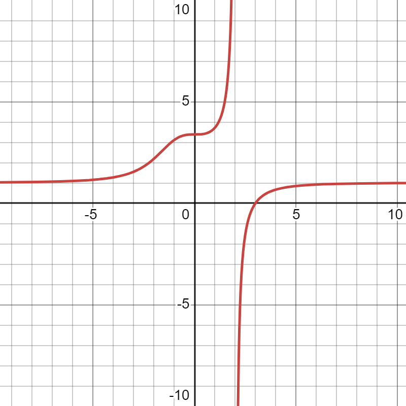
3. First, notice that the denominator can be seen as \( (x^2)^2 + 2 (x^2) + 1 \), which can be factored as a perfect square to get \( r(x) = \dfrac{1}{(x^2 + 1)^2} \). Looking at the numerator, we see it can never be 0 because it's always 1, so there are no roots! Looking at the denominator, we ask ourselves if any \(x\)-value would cause division by zero... Nope! Everything going on here is strictly positive. So there's also no vertical asymptote. If you're curious, this guy looks like this:

Algebraically identify any roots and vertical asymptotes of the rational functions.
1. \( f(x) = \dfrac{x^2+6x+8}{x^3+3x^2-x-3} \)
2. \( g(x) = \dfrac{x^2+x+2}{x^2 - 2x + 1} \)
3. \( h(x) = \dfrac{x^3 + x^2}{x-2} \)
- Answer
-
- (Factor by grouping in denominator.) Roots: \(x = -2, -4 \). V.A.s: \(x = -3, x = -1, x = 1 \).
- Roots: no real roots. V.A.s: \( x = 1 \).
- Roots: \(x = 0, -1\). V.A.s: \(x = 2\).
Graphically, identify any roots, vertical asymptotes, and horizontal asymptotes.
 |
 |
 |
 |
| 1. | 2. | 3. | 4. |
- Answer
-
- Roots: \( x = -2 \). V.A.: \(x = 3 \). H.A.: \( y = 1\).
- Roots: \( x = 3 \). V.A.: \( x = 2 \). H.A.: \( y = 1\).
- Roots: none. V.A.s: \( x = -2, \) \( x = 2\). H.A.: \( y = 1\).
- Roots: \(x = 1\). V.A.s: \( x = 0, x = -3\). H.A.: \( y = 0 \).
We're going to get serious about algebraically finding horizontal asymptotes in the next section, when we talk about limits. For now, I just want to be sure you can deal with these functions if they come up using a couple of tools. One thing you might need to do at some point is translate from a rational expression to the equivalent quotient-and-remainder version. You'll use polynomial long division to achieve this. This is productive if (a) the degree of the top is larger than the degree of the bottom, or (b) the degrees are the same. If the degree of the bottom is larger, there's nothing to do with the division.
Write the rational function \(f(x) = \dfrac{p(x)}{d(x)} \) as \( f(x) = q(x) + \dfrac{ r(x)}{d(x)} \).
1. \( f(x) = \dfrac{ x^2 + 3x + 2 }{x-4} \)
2. \( f(x) = \dfrac{ x^2 - 4 } {x^2 - 9} \)
3. \( f(x) = \dfrac{ 1}{x^4 + 2x^2 + 1 } \)
Solution
1. Simply perform the division:
\begin{array}{r}
x+7\phantom{)} \\
x-4{\overline{\smash{\big)}\,x^2+3x+2\phantom{)}}}\\
\underline{-~\phantom{(}(x^2-4x)\phantom{-b)}}\\
0+7x+2\phantom{)}\\
\underline{-~\phantom{()}(7x-28)}\\
0+30\phantom{)}
\notag
\end{array}
We get \( f(x) = x+7 + \dfrac{30}{x-4} \)
2. You can either do long division, which is a little funky:
\begin{array}{r}
1\phantom{)} \\
x^2-9{\overline{\smash{\big)}\,x^2+0x-4\phantom{)}}}\\
\underline{-~\phantom{(}(x^2\phantom{+0x}-9)}\\
0+5\phantom{)}\\ \notag
\end{array}
or just notice that \( - 4 = -9 + 5 \), do a sneaky replacement, and split the fraction:
\[ f(x) = \dfrac{ x^2 - 4 } {x^2 - 9} = \dfrac{ x^2 \textcolor{red}{-9+5} } {x^2 - 9} = \dfrac{ x^2 - 9 } {x^2 - 9} + \dfrac{ 5} {x^2 - 9} = 1 + \dfrac{ 5} {x^2 - 9} \notag \]
Either way, you get the same thing.
3. This is already in the desired form actually, because if you try to do long division, you will find \( q(x) = 0\) and \(r(x) = f(x)\).
Go back and try it yourself on the rational functions from Exercise 1! (Check your answers: 1. already in the form; 2. \(1+\frac{3x+1}{x^2-2x+1}\); 3. \(x^2+3x+6 + \frac{12}{x-2} \).)
Partial Fraction Decomposition
Another way to rewrite rational functions in a useful way (this comes up in Calc II and Differential Equations, for example) uses a special technique called partial fractions. Polynomial long division above allowed us to split up a big rational expression as long as the degree of the top wasn't smaller than the degree of the bottom. The partial fractions method allows to deal with that left-out situation! I want to introduce you to it here at a simplified level. The idea is to kinda undo the process of getting a common denominator. In numbers, it would be like writing:
\[ \frac{41}{30} = \frac{ 1}{2} + \frac{2}{3} + \frac{ 1}{5} \notag \]
What we want is to split a rational expression into several fractions whose denominators are factors of the original denominator, like this:
\[ \frac{ x+1}{x(x-1)(x+2)} = \frac{A}{x} + \frac{B}{x-1} + \frac{C}{x+2} \notag \]
Our mission is to figure out what the numerators \(A, B,\) and \(C\) need to be to make this equation true. The basic process is simply to clear the denominators and consider like terms separately. See the example below.
Find \(A, B,\) and \(C\) to write \( f(x) = \dfrac{ x+1}{x(x-1)(x+2)} = \dfrac{A}{x} + \dfrac{B}{x-1} + \dfrac{C}{x+2} \).
Solution
First, multiply through the entire equation carefully by the left hand side's whole denominator, which will have the effect of clearing all denominators when you distribute through the right hand side.
\[ \textcolor{red}{x(x-1)(x+2)} \cdot \dfrac{ x+1}{x(x-1)(x+2)} = \left( \dfrac{A}{x} + \dfrac{B}{x-1} + \dfrac{C}{x+2} \right) \cdot \textcolor{red}{x(x-1)(x+2)} \notag \]
This boils down to \( x+1 = A(x-1)(x+2) + Bx(x+2) + Cx(x-1) \). Next, expand everything as much as possible by FOILing and distributing.
\[ x+1 = Ax^2 + Ax - 2A + Bx^2 + 2Bx + Cx^2 - Cx \notag \]
Now, we compare the coefficients of like terms on both sides of the equation. For example, on the left we have NO \(x^2\) terms, but on the right there are \( Ax^2 + Bx^2 + Cx^2 \). In order for these to turn out the same, I must have \( 0 = A + B + C \). Next, compare the \(x\) terms. On the left, there is a single \(x\), and on the right we have \( Ax + 2Bx - Cx \). This means we must have \( 1 = A + 2B - C \). Finally, compare the constant terms. On the left, we have \(1\), and on the right, \( -2A \). Our last equation is \( 1 = -2A\).
Everything has boiled down to a system of equations!
\[ \begin{cases} A + B + C &= 0 \\ A + 2B - C &= 1 \\ -2A & = 1 \end{cases} \notag \]
Solving this system using the methods of Section 3.5, we find \(A = -\frac{1}{2}, B = \frac{2}{3}, C = -\frac{1}{6} \). Thus, we can write
\[ \dfrac{ x+1}{x(x-1)(x+2)} = -\dfrac{1}{2} \cdot \dfrac{1}{x} + \dfrac{2}{3} \cdot \dfrac{1}{(x-1)} - \dfrac{1}{6} \cdot \dfrac{1}{(x+2)} \notag \]
1. Use partial fractions to write \(f(x) = \dfrac{2x}{x^2+5x + 6} \) as a sum of terms whose denominators are linear factors of the denominator of \(f\). Meaning, factor the denominator first, and then find \( A\) and \(B\) such that \( f(x) = \dfrac{2x}{x^2+5x + 6} = \dfrac{A}{x+3} + \dfrac{B}{x+2}\).
2. Use partial fractions to write \( f(x) = \dfrac{ x-3}{x^3 - x} \) as a sum of terms whose denominators are linear factors of the denominator of \(f\).
- Answer
-
1. \( f(x) = \dfrac{2x}{x^2+5x + 6} = \dfrac{6}{x+3} - \dfrac{4}{x+2}\)
2. \( f(x) = \dfrac{ x-3}{x^3 - x} = \dfrac{3}{x} - \dfrac{2}{x+1} - \dfrac{1}{x-1}\)
The above method works whenever all the factors in the denominator are linear and distinct. In the case of repeated or irreducible quadratic factors, things get a little more complicated. I leave that for when it becomes necessary in later courses, but if you're really curious you can check out the table at this link now!
Polynomial and Rational Inequalities
The methods in this section are going to be very similar to the number line process from Section 3.2, if you want to review that real quick. If you're all set, read on.
By looking at a graph of \(y = f(x)\), it's pretty easy to assess an inequality of the form, say, \(f(x) > 0\), or \( f(x) \leq 0\). This is simply a matter of the function values, aka \(y\)-values, being positive versus negative. Well, if you have positive \(y\)-coordinate, you're above the \(x\)-axis, and if you have negative \(y\)-coordinate, you're below it. So we can easily read off the zones that provide the solution to such an inequality. See the graphical example below.


Notice that the only way for a polynomial function to change from negative to positive values or vice versa is for it to pass through the \(x\)-axis, at the location of a root! So the roots of the function are the signpost points around which we will base our analysis. Here's the process:
To solve a polynomial inequality:
- Move all the terms to one side and get 0 on the other.
- Factor the polynomial into linear factors and irreducible quadratic factors, and find the real roots.
- Make a number line, divided into zones (intervals) by the roots.
- In each zone, determine whether the function is positive or negative by using logic or testing points and comparing the signs of the factors.
- Report the desired zones as intervals, based on the inequality sign.
Solve the polynomial inequality \( 2x^3 - x^2 - 2x > -1 \).
Solution
1. We move everything to the left side: \( 2x^3 - x^2 - 2x + 1 > 0 \).
2. This polynomial was factored in Example 4 of Section 5.4, so refer back to that if you get stuck. We get \( (2x-1)(x-1)(x+1) > 0 \). The roots are \(x = -1, \frac{1}{2}, 1 \).
3. We set up the number line, split at the roots. (The red 0 is just for reference.)
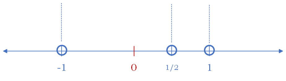.png?revision=1&size=bestfit&width=565&height=160)
4. In each zone, we determine the sign of the polynomial. For the first zone, you could try plugging in \(-2\) to see that the factors \( (\text{neg})(\text{neg})(\text{neg})\) will result in a negative number. For the second zone, plug in 0, which would give the factors \( (\text{neg})(\text{neg})(\text{pos}) = \text{pos}\). For the third zone, we find \( (\text{pos})(\text{neg})(\text{pos}) = \text{neg} \). For the last zone, we find \( (\text{pos})(\text{pos})(\text{pos}) = \text{pos} \). Label the zones.
.png?revision=1&size=bestfit&width=559&height=159)
5. We are looking for the positive zones because we want to be greater than 0. Since the inequality is strict, we won't include the endpoints of the intervals. Our final answer is the list of intervals: \( \left( -1, \frac{1}{2} \right) \cup (1, \infty) \).

The process is extremely similar for solving rational inequalities. The only difference to account for is that it's possible for a rational function to jump over the \(x\)-axis without passing through it, due to the vertical asymptotes. See below, where the graph is positive on one side of the V.A. \(x = -2\) and negative when you hop to the other side, etc.

To solve a rational inequality:
- Move all the terms to one side into a single giant fraction and get 0 on the other.
- Factor the numerator and the denominator. Identify the points of interest where either the numerator or the denominator are zero. (Basically, roots of the top poly and roots of the bottom poly.)
- Make a number line, divided into zones (intervals) by the points of interest.
- In each zone, determine whether the function is positive or negative by using logic or testing points and comparing the signs of the factors.
- Report the desired zones as intervals, based on the inequality sign. Test the endpoints carefully to see if they should be included, because the function may not be defined at some of them!
Solve the rational inequality \( \dfrac{4}{x+2} + 1 \leq x \).
Solution
1. We move all terms over, get a common denominator, and combine into a single rational expression.
\[ \dfrac{4}{x+2} + 1 - x \leq 0 \quad \rightarrow \quad \dfrac{4}{x+2} + \dfrac{ (1-x)(x+2)}{x+2} \leq 0 \quad \rightarrow \quad \dfrac{ 4 + (1-x)(x+2)}{x+2} \leq 0 \notag \]
2. We expand and simplify the numerator so that we can factor it. The denominator is already a linear factor.
\[ \dfrac{ 4 - x^2 - x + 2}{x+2} = \dfrac{ -(x^2+x-6)}{x+2} = \dfrac{ -(x-2)(x+3)}{x+2} \notag \]
The points of interest are \(x = -3, -2, 2 \).
3. We make the number line.

4. In the first zone, we imagine plugging in \(-4\) and deduce that the rational expression will be \( \dfrac{ -(\text{neg})(\text{neg})}{\text{neg}} = \text{pos}\). In the second zone, \( \dfrac{ -(\text{neg})(\text{pos})}{\text{neg}} = \text{neg}\). In the third zone, \( \dfrac{ -(\text{neg})(\text{pos})}{\text{pos}} = \text{pos}\). In the last zone, \( \dfrac{ -(\text{pos})(\text{pos})}{\text{pos}} = \text{neg}\).

5. We want to be less than or equal to 0, so we take the negative zones and test the endpoints. At \(x = -3\), the expression equals 0, so that's fine. At \(x = -2\), the expression is not defined, so we leave that out! At \(x = 2\), the expression is 0 again. Our final answer is \( [-3,-2) \cup [2,\infty) \).

Now you try!
Solve the inequalities.
1. \( x^3 - 4x \geq 0 \)
2. \( x^2 - 4 < \dfrac{1}{x^2 - 1} \)
3. \( \dfrac{x^2+2x}{x^2-3x+2} \leq 0 \)
4. \( \dfrac{2x}{x+1} > x^2 \)
- Answer
-
- \( [-2, 0] \cup [2, \infty) \)
- \( (-2,-1) \cup (1,2) \)
- \( [-2, 0] \cup (1,2) \)
- \( (-2, -1) \cup (0,1) \)
Throughout this section, we have assumed that our rational functions are fully reduced. Of course, if you construct or come across rational functions in the course of your math career, this may not be the case yet! When a function is defined using a rational expression that is not fully reduced, it produces a hole or removable discontinuity in the graph. You will investigate this in the exercises section!