7.1 Exponential Functions

Learning Objectives

By the end of this section, you will be able to:

• recognize exponential functions, their important features, and their graphs
• recognize transformations of exponential functions and their graphs
• sketch the graph of an exponential function
• evaluate exponential functions and use technology to solve problems

As you've probably deduced from the name, exponential functions involve raising something to some kind of power. We've seen functions where a variable is raised to a plain ol' number power already; those are polynomials like \( p(x) = x^3 \). Well, this is the other way around. This time, we're taking a plain ol' number as the base and putting the variable upstairs in the exponent. Like the functions \( f(x) = 3^x\) or \(g(x) = 17^x \), or even \( \exp(t) = e^t \), which uses the number \( e \approx 2.718...\) as the base!

We're secretly making a claim here that we know how to raise a number to ANY real number power, because we want to say that \(x\) can be anything. We know how to do integer powers and rational powers, but how do you deal with irrational numbers? A calculator can handle it, by simply rounding off the decimal approximation of an irrational number somewhere, and computing that rational number power instead. In practice, you can get "close enough" for your various purposes using technology to do this approximation technique.

Here's some good news: All of the power rules that we know already still apply!

Technology Note: when you need to type exponents into various calculators/websites, you will generally use the carat symbol ^ (shift+6 on a keyboard). If your power is very complicated, you'll want to also use parentheses. For example, to enter \( 2^{-\sqrt{5}} \) into WolframAlpha, you can type "2^(-sqrt(5))" and it will understand.

Exponential Functions

The exponential function with base \(a\) is defined by \( f(x) = a^x\), for all real numbers \( x\), where \( a > 0\) and \(a \neq 1\).

Fun facts about exponential functions:

• We don't allow \(a = 1\) because \(1^x\) is always 1, giving a super boring constant function \(f(x) = 1\).
• We don't allow negative bases because raising negative numbers to even (and some fractional) powers is a mess for the real numbers.
• The domain of an exponential function is all real numbers.

Exponential functions are very sensitive. A small change in the variable can cause significant change in the function value. For example, if \(f(x) = 8^x\), consider

\(x\)-value	0	1	2	3	4
\(f(x)\)	\(8^0 = 1\)	\(8^1 = 8\)	\(8^2 = 64\)	\(8^3 = 512 \)	\(8^4 = 4096\)

Going from \(x = 2\) to \(x = 3\) doesn't feel like much, but the function value shoots from 64 all the way to 512.

When you raise a base \(a > 1\) to bigger and bigger powers, the results increase, just like the example above with \(a = 8\). Let's see some graphs.

Observations:

• All \( f(x) = a^x\) pass through the point \( (0,1) \). This makes sense because anything raised to the 0 is 1, so \(f(0) = a^0 = 1\), regardless of what \(a\) is.
• There's no reason a base has to be a whole number! Recall the special number \(e \approx 2.718 \). You can use him as a base number, and you can see that his graph lies between \(f(x) = 2^x\) and \(g(x) = 3^x\), just as \( 2< 2.718 < 3 \).
• On the left side of the graph, as \(x \rightarrow -\infty\), the graphs hug a horizontal asymptote \( y = 0\). This makes sense because plugging in negative numbers as powers produces smaller and smaller numbers. For example,
  \[ 2^{-1} = \frac{1}{2}, \quad \quad 2^{-2} = \frac{1}{4}, \quad \quad 2^{-5} = \frac{1}{32}, \quad ... \notag \]
• These functions are always positive! The graph never crosses the \(x\)-axis. Why? Is there any option for \(x\) such that \(a^x = 0\)?
• Since \(a^1 = a \) for any \(a\), you can see that they each pass through the point \( (1,a)\) matching their base. For example, \(f(x) = 2^x\) passes through \( (1,2)\).
• Looking out at end behavior as \(x \rightarrow \infty\), the bigger the base, the steeper the function (the faster it grows).

On the other hand, if \(0< a < 1\), raising to higher and higher powers causes the function value to decrease. For example, consider raising \(a= \frac{1}{2} \) to powers...

\[ \left( \frac{1}{2} \right)^{-1} = 2, \quad \quad \left( \frac{1}{2} \right)^0 = 1, \quad \quad \left( \frac{1}{2} \right)^1 = \frac{1}{2} , \quad \quad \left( \frac{1}{2} \right)^2 = \frac{1}{4}, \quad ... \notag \]

Observations (reason through them as above):

• The graphs all still pass through \( (0,1) \).
• The graphs hug a horizontal asymptote \( y = 0\), this time as \(x \rightarrow \infty\) to the right.
• The functions are still always positive (above the \(x\)-axis).
• The functions still pass through the point \( (1,a)\) where \(a\) is their base. They also pass through the point \( \left(-1, \frac{1}{a} \right) \), which is often easier to see on the graph. For example, \( f(x)\) above passes through \( (-1, 2) \).

There's one more thing I want to call out, which I've hinted at in the graph above, labeling \(h(x) = e^{-x} = \frac{1}{e}^x \). Remember your power rules! There is a relationship between the functions \(f(x) = a^x\) and \( g(x)= \left( \frac{1}{a}\right)^x \).

\[ g(x) = \left( \frac{1}{a}\right)^x = \frac{1}{a^x} = a^{-x}= f(-x) \notag \]

You can transform \(f\) into \(g\) by replacing the input \(x\) with \(-x\), which we recall from function transformations causes a reflection about the \(y\)-axis. Observe below.

To sum up,

• If \(a > 1\), the function is increasing (graph going uphill from left to right). If \( 0 < a< 1\), the function is decreasing (graph going downhill from left to right). These trends are called exponential growth or exponential decay, respectively.
• End behavior for \(a > 1\): As \(x \rightarrow -\infty\), the graph hugs a horizontal asymptote at the \(x\)-axis. As \(x \rightarrow \infty\), the graph shoots up rapidly, and the bigger the base, the faster the growth.
• End behavior for \( 0<a<1\): As \(x \rightarrow -\infty\), the graph is blowing up to the left. As \(x \rightarrow \infty\), the graph hugs the horizontal asymptote at the \(x\)-axis forever.
• All exponential functions pass through \( (0,1)\) as well as \( (1,a)\), for whatever their base \(a\) is.
• The function values are always positive, aka above the \(x\)-axis, aka the range is \( (0, \infty) \).
• For \( f(x) = a^x\) and \( g(x) = \left( \frac{1}{a}\right)^x \), note that \( g(x) = \left( \frac{1}{a}\right)^x = \frac{1}{a^x} = a^{-x} = f(-x) \).

Test your understanding with the exercises below.

Exercise \(\PageIndex{1}\)

Answer True/False:

1. The function \( f(x) = x^7\) is exponential with base 7.
2. The function \( f(x) = 7^x \) is exponential with base 7.
3. The function \( f(x) = 4^x\) is a horizontal reflection across the \(y\)-axis of the function \( g(x) = 4^{-x} \).
4. The function \( f(x) = 4^x\) is a horizontal reflection across the \(y\)-axis of the function \( g(x) = \left( \frac{1}{4} \right)^x \).
5. The graph of \(f(x) = (1.5)^x\) is increasing.
6. The graph of \( f(x) = (0.25)^x\) is decreasing.
7. The graph of \( f(x) = 3^x \) is decreasing.
8. As \(x \rightarrow \infty\), the graph of \( f(x) = 2^x \) is steeper (faster growing) than the graph of \( g(x) = 3^x \).
9. As \(x \rightarrow \infty\), the graph of \( f(x) = 5^x \) is steeper (faster growing) than the graph of \(g(x) = e^x \).
10. The graph of \( f(x) = 6^x\) passes through \( (1,6) \).
11. The graph of \(f(x) = 3^x \) passes through \( (3,1)\).
12. The graph of \(f(x) = a^x\) passes through \( (0,1)\) for any base \(a\).
13. The graph of \(f(x) = a^x\) passes through \( (1,0)\) for any base \(a\).
14. There exists a value of \(x\) such that \( a^x < 0 \) for any base \(a\).

Answer

1. False. That's a polynomial (monomial) with degree 7.
2. True.
3. True.
4. True, this is equivalent to the previous statement.
5. True, the base is bigger than 1.
6. True, the base is smaller than 1.
7. False.
8. False, the bigger the base, the faster the growth.
9. True, 5 is a bigger base than \(e \approx 2.71...\).
10. True, \(f(1) = 6 \).
11. False, it passes through \( (1,3) \) though. At \(x = 3\), \(f(3) = 9\).
12. True, \(a^0 = 1\) for any \(a\).
13. False, \(a^1 \neq 0\).
14. False, the function \(f(x) = a^x\) is always positive.

Exercise \(\PageIndex{2}\)

Match the exponential functions with their graphs.

1.	2.	3.	4.
\( f(x) = e^x\)	\( g(x) = 2^x \)	\( h(x) = \left(\frac{1}{2}\right)^x \)	\( p(x) = e^{-x} \)

Answer

1. \(h\)
2. \(f\)
3. \( g\)
4. \( p\)

Transformations of Exponential Functions

Recall from our study of function transformations that you can...

• Shift a function vertically by changing from \( f(x)\) to \( f(x) \pm k\).
• Shift a function horizontally by changing from \( f(x)\) to \(f(x\pm k) \).
• Stretch or shrink a function vertically by changing from \( f(x)\) to \( k f(x) \).
• Stretch or shrink a function horizontally by changing from \( f(x)\) to \( f(kx)\).
• Reflect a function across the \(y\)-axis by changing from \( f(x) \) to \( f(-x)\).
• Reflect a function across the \(x\)-axis by changing from \( f(x)\) to \( - f(x)\).

Although the definition of "the" exponential functions above is a simple \( f(x) = a^x\), you will hear people use the term "exponential function" for anything that looks like the guy below, where \(c_0, c_1, c_2,\) and \(c_3\) are all constants that have shown up due to transformations.

\[ f(x) = c_1 a^{c_2 x+c_3} + c_0 \notag \]

(This would be like taking \(a^x\) and doing a horizontal shift then stretch, then a vertical stretch then shift... if \(c_1\) or \(c_2\) are negative, maybe there was a reflection in there, yikes...)

We will see a whole bunch of functions like this when we practice application problems. For now, I want you to apply your previous knowledge to match graphs to their functions.

Example \(\PageIndex{1}\)

Give the function whose graph is shown. I've marked some signal points to use in the reasoning. I will give you matching in your own exercise, but this will help you understand the process.

1.	2.	3.

Solution

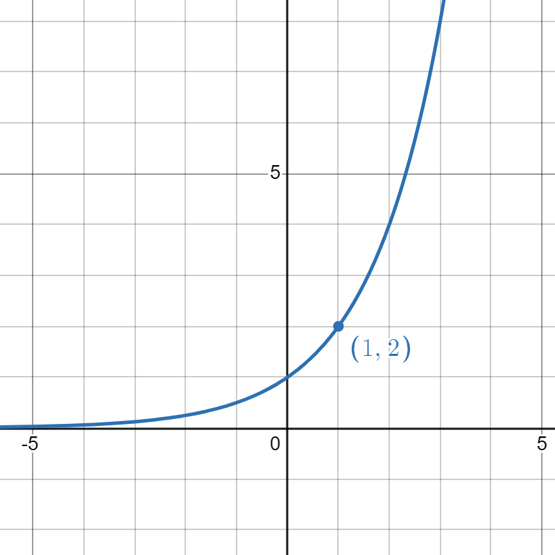
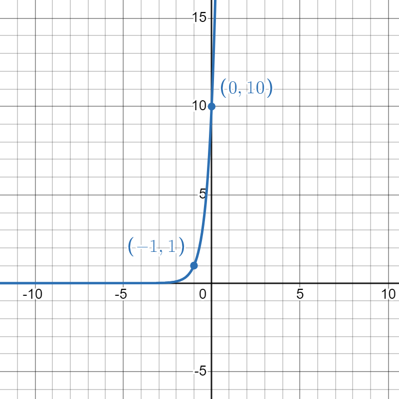
1. The easiest thing to look out for first is where the horizontal asymptote has moved to. It used to be at \(y = 0\) but now it's at \(y = -3\), which is a vertical shift down by \(3\), so I start out thinking about "\(a^x - 3 \)." Normally, the graph passes through the point \( (0,1)\), and I see now it passes through \( (0, -2) \), so that's consistent with the vertical shift. Before the shift, the point \( (1,-1) \) would have been at \( (1, 2) \), and that looks like \( (1,a)\) for \(a = 2\). So I think I'm looking at \( f(x) = 2^x - 3 \). Let's check the other point, \( (2,1)\) by plugging in \(x = 2\). We have \( f(2) = 2^2 - 3 = 1,\) yep! Note: if a vertical shift is involved, it's totally possible for a transformed function like this to take negative values. It's just the \(a^x\) guys that are guaranteed to be always positive.

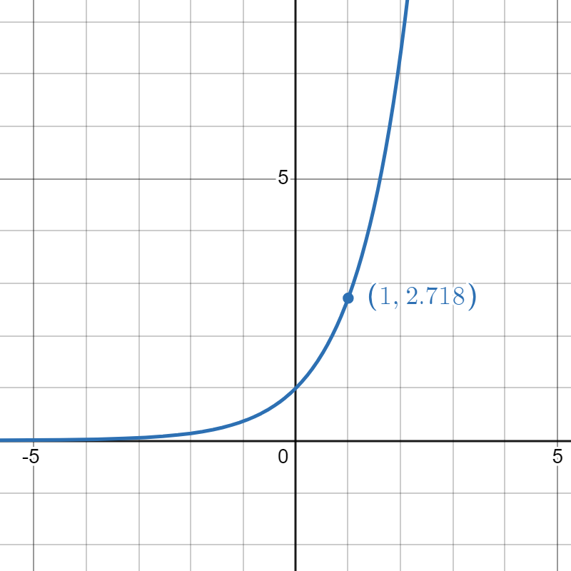
2. First, the horizontal asymptote is still at 0, so I don't have a vertical shift. That point \( (1, e^2) \) is an interesting choice of call-out... What kind of function of the form \(a^{kx}\) could produce \(e^2\) when \(x = 1\)? Well, the \(a\) better be base \(e\), and \(k = 2\) would work! This function is \(f(x) = e^{2x} \). Visually, this looks like \(e^x\) got a horizontal squish.

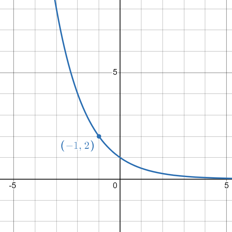
3. Again, no vertical shift happening. Now, usually the function should pass through \( (0,1)\), but it looks like that point has shifted horizontally over to \( (-1,1)\). That's a horizontal shift to the left by 1. That means the point \( (0,10)\) was originally \( (1,10)\), and who passes through that? We must have started with \( 10^x\) and then performed the shift left. That gives us \( f(x) = 10^{x+1} \).

Exercise \(\PageIndex{3}\)

Match the graphs to their functions.

1.	2.	3.	4.
\( f(x) = e^{-x} \)	\( g(x) = -e^x\)	\( h(x) = 3^x + 1 \)	\(p(x) = 2^{x-3} \)

Answer

1. Remember that \(e \approx 2.718...\) so that point is \( (1,-e) \). This graph looks exactly like \(y = e^x\) reflected over the \(x\)-axis, which would become \(-e^x\). Must be \(g\).
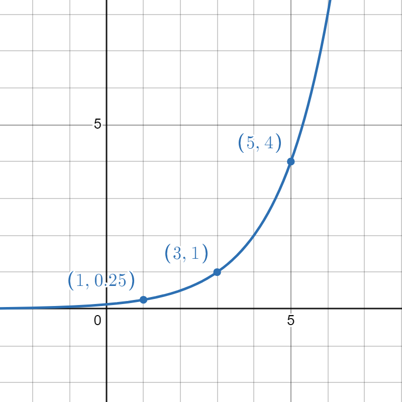
2. No vertical shift here. Usually we pass through \( (0,1)\) but this time, we pass through \( (3,1)\). That looks like a horizontal shift by 3 to the right. Let's hypothesize "\(a^{x-3}\)" and see what would satisfy the point \( (5,4)\). We want to get \(4\) when plugging in \(x = 5\), so what would make
   \[ a^{5-3} = a^2 = 4 \notag \]
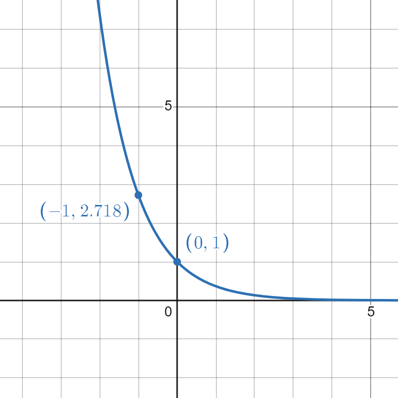
   be true? The base \(a = 2\) will do that! If you want to double check, try plugging in \( x = 1\) to confirm the point \( (1, 0.25) \). This goes with \(p\).
3. Aha, \(e\) again! This time, we've had a reflection over the \(y\)-axis. That happens if you replace \(x\) with \( (-x)\) in the function \(e^x\). So this goes with \(f\).
4. The asymptote has moved from the \(x\)-axis up by 1, so we have a vertical shift. We expect something like "a^x + 1" and there's only one function that looks like that! Well, also only one function left to choose, lol. You can confirm that \(h\) will pass through the given points.

If you ever find yourself in a pinch (marooned on a deserted island? jumped in an alleyway by a mathematician?) needing to graph an exponential function by hand, here's what I recommend.

To sketch the graph of an exponential function,

1. Find the \(y\)-intercept by plugging in \(x = 0\) and drop that point in.
2. Compute a couple more easy-to-evaluate points, like plugging in \(x = \pm 1, \pm 2\).
3. Check if there's a "\(+k\)" of some sort on the end of the whole function. That'll be a vertical shift. You could draw in your horizontal asymptote.
4. Check if there's a negative somewhere causing a reflection.
5. Use all that knowledge to connect the dots in the general shape you expect for an exponential, so...a big swoop.

Working With Exponential Functions

If you need to simplify an exponential expression, simply apply your power rules! For very simple (or very well-cooked) problems, you can evaluate exponential functions by hand, but for more complicated functions or ugly numbers, you will need a calculator or technology of some sort. Let's practice.

Example \(\PageIndex{2}\)

Without using technology, simplify the functions (first), and (then) evaluate them at the given \(x\)-values.

1. \( f(x) = 3^x 9^x +1 \), at \( x = -1, 0, 1 \).
2. \( g(x) = 2(2^{x+1}) \), at \( x = -1, 0, 1, 2\).
3. \( h(x) = \dfrac{3^x}{6} - 2 \), at \(x = -1, 0, 1, 2 \).

Solution

1. First, simplify by using power rules (I'm going to break this down this time, but if this is not second nature to you, review power rules asap)...
\[ f(x) = 3^x \textcolor{red}{(3^2)}^x + 1 = 3^x 3^{\textcolor{red}{2x}} + 1 = 3^{\textcolor{red}{x+2x}} + 1 = 3^{3x} + 1 \quad \text{ or } \quad = 27^x + 1 \notag \]
Then just plug in to find \( f(-1) = \frac{1}{27}+1 = \frac{28}{27} \), \( f(0) = 27^0 + 1 = 2\), and \( f(1) = 28\).

2. First, simplify as \( g(x) = 2^1 2^{x+1} = 2^{x+2} \) and then evaluate \( g(-1) = 2\), \( g(0) = 4 \), \( g(1) = 8\), and \( g(2) = 16 \).

3. First, simplify as
\[ h(x) = \dfrac{3^x}{2\cdot 3} - 2 = \dfrac{1}{2} \cdot 3^x 3^{-1} - 2 = \frac{1}{2}\cdot 3^{x-1} - 2 \notag \]
Then evaluate \( h(-1) = \frac{1}{2}(3^{-2}) - 2 = \frac{1}{18} - 2 = \frac{1}{18} - \frac{36}{18} =- \frac{35}{18} \), \(h(0) = -\frac{11}{6}\), \(h(1)= -\frac{3}{2} \), and \( h(2) = -\frac{1}{2} \).

Exercise \(\PageIndex{4}\)

Without using technology, simplify and evaluate the functions at the given \(x\)-values.

1. \( f(x) = 2^x + 2^x - 2 \), at \(x = -1, 0, 1, 2\).
2. \( g(x) = \dfrac{ 9^x}{81^x} \), at \( x = -1, 0, 1, 2\).
3. \( h(x) = 5(1+0.5)^x \), at \( x = -1, 0, 1, 2 \).

Answer

1. \( f(x) = 2(2^x) - 2 = 2^{x+1} - 2 \) and \(f(-1) = -1\), \(f(0) = 0 \), \(f(1) = 2\), \(f(2) = 6 \).

2. \( g(x) = \dfrac{1}{9^x} \) or \(9^{-x} \), and \( g(-1) = 9\), \(g(0) = 1 \), \(g(1) = \frac{1}{9} \), \(g(2) = \frac{1}{81}\).

3. \( h(x) = 5 \left( \frac{3}{2} \right)^x \) and \( h(-1) = \frac{10}{3} \), \( h(0) = 5 \), \(h(1) = \frac{15}{2}\), \( h(2) = \frac{45}{4} \).

Exercise \(\PageIndex{5}\)

Using technology, fill in the table of values for the function \(f(t) = 100\left(1+\frac{0.12}{2}\right)^{2t} \). (I recommend simplifying first.) Round to two decimal places if needed.

\(t\)	\(f(t)\)	\(t\)	\(f(t)\)
0		5
1		10
2		20
3		100

Answer

Simplified, \(f(t) = 100 (1.06)^{2t}\).

Let me teach you a technology trick for this kind of thing (for when you're allowed to use technology, of course, not for cheating). Go to wolframalpha.com and type in "table of values 100(1.06)^(2t) for t = 0, 1, 2, 3, 5, 10, 20, 100" and hit Enter. You're welcome.

\(t\)	\(f(t)\)	\(t\)	\(f(t)\)
0	100	5	179.09
1	112.36	10	320.71
2	126.25	20	1028.57
3	141.85	100	11,512,600