
6.4: Areas of Surfaces of Revolution
- Page ID
- 8165
\( \newcommand{\vecs}[1]{\overset { \scriptstyle \rightharpoonup} {\mathbf{#1}} } \)
\( \newcommand{\vecd}[1]{\overset{-\!-\!\rightharpoonup}{\vphantom{a}\smash {#1}}} \)
\( \newcommand{\id}{\mathrm{id}}\) \( \newcommand{\Span}{\mathrm{span}}\)
( \newcommand{\kernel}{\mathrm{null}\,}\) \( \newcommand{\range}{\mathrm{range}\,}\)
\( \newcommand{\RealPart}{\mathrm{Re}}\) \( \newcommand{\ImaginaryPart}{\mathrm{Im}}\)
\( \newcommand{\Argument}{\mathrm{Arg}}\) \( \newcommand{\norm}[1]{\| #1 \|}\)
\( \newcommand{\inner}[2]{\langle #1, #2 \rangle}\)
\( \newcommand{\Span}{\mathrm{span}}\)
\( \newcommand{\id}{\mathrm{id}}\)
\( \newcommand{\Span}{\mathrm{span}}\)
\( \newcommand{\kernel}{\mathrm{null}\,}\)
\( \newcommand{\range}{\mathrm{range}\,}\)
\( \newcommand{\RealPart}{\mathrm{Re}}\)
\( \newcommand{\ImaginaryPart}{\mathrm{Im}}\)
\( \newcommand{\Argument}{\mathrm{Arg}}\)
\( \newcommand{\norm}[1]{\| #1 \|}\)
\( \newcommand{\inner}[2]{\langle #1, #2 \rangle}\)
\( \newcommand{\Span}{\mathrm{span}}\) \( \newcommand{\AA}{\unicode[.8,0]{x212B}}\)
\( \newcommand{\vectorA}[1]{\vec{#1}} % arrow\)
\( \newcommand{\vectorAt}[1]{\vec{\text{#1}}} % arrow\)
\( \newcommand{\vectorB}[1]{\overset { \scriptstyle \rightharpoonup} {\mathbf{#1}} } \)
\( \newcommand{\vectorC}[1]{\textbf{#1}} \)
\( \newcommand{\vectorD}[1]{\overrightarrow{#1}} \)
\( \newcommand{\vectorDt}[1]{\overrightarrow{\text{#1}}} \)
\( \newcommand{\vectE}[1]{\overset{-\!-\!\rightharpoonup}{\vphantom{a}\smash{\mathbf {#1}}}} \)
\( \newcommand{\vecs}[1]{\overset { \scriptstyle \rightharpoonup} {\mathbf{#1}} } \)
\( \newcommand{\vecd}[1]{\overset{-\!-\!\rightharpoonup}{\vphantom{a}\smash {#1}}} \)
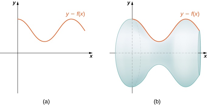
\(\newcommand{\avec}{\mathbf a}\) \(\newcommand{\bvec}{\mathbf b}\) \(\newcommand{\cvec}{\mathbf c}\) \(\newcommand{\dvec}{\mathbf d}\) \(\newcommand{\dtil}{\widetilde{\mathbf d}}\) \(\newcommand{\evec}{\mathbf e}\) \(\newcommand{\fvec}{\mathbf f}\) \(\newcommand{\nvec}{\mathbf n}\) \(\newcommand{\pvec}{\mathbf p}\) \(\newcommand{\qvec}{\mathbf q}\) \(\newcommand{\svec}{\mathbf s}\) \(\newcommand{\tvec}{\mathbf t}\) \(\newcommand{\uvec}{\mathbf u}\) \(\newcommand{\vvec}{\mathbf v}\) \(\newcommand{\wvec}{\mathbf w}\) \(\newcommand{\xvec}{\mathbf x}\) \(\newcommand{\yvec}{\mathbf y}\) \(\newcommand{\zvec}{\mathbf z}\) \(\newcommand{\rvec}{\mathbf r}\) \(\newcommand{\mvec}{\mathbf m}\) \(\newcommand{\zerovec}{\mathbf 0}\) \(\newcommand{\onevec}{\mathbf 1}\) \(\newcommand{\real}{\mathbb R}\) \(\newcommand{\twovec}[2]{\left[\begin{array}{r}#1 \\ #2 \end{array}\right]}\) \(\newcommand{\ctwovec}[2]{\left[\begin{array}{c}#1 \\ #2 \end{array}\right]}\) \(\newcommand{\threevec}[3]{\left[\begin{array}{r}#1 \\ #2 \\ #3 \end{array}\right]}\) \(\newcommand{\cthreevec}[3]{\left[\begin{array}{c}#1 \\ #2 \\ #3 \end{array}\right]}\) \(\newcommand{\fourvec}[4]{\left[\begin{array}{r}#1 \\ #2 \\ #3 \\ #4 \end{array}\right]}\) \(\newcommand{\cfourvec}[4]{\left[\begin{array}{c}#1 \\ #2 \\ #3 \\ #4 \end{array}\right]}\) \(\newcommand{\fivevec}[5]{\left[\begin{array}{r}#1 \\ #2 \\ #3 \\ #4 \\ #5 \\ \end{array}\right]}\) \(\newcommand{\cfivevec}[5]{\left[\begin{array}{c}#1 \\ #2 \\ #3 \\ #4 \\ #5 \\ \end{array}\right]}\) \(\newcommand{\mattwo}[4]{\left[\begin{array}{rr}#1 \amp #2 \\ #3 \amp #4 \\ \end{array}\right]}\) \(\newcommand{\laspan}[1]{\text{Span}\{#1\}}\) \(\newcommand{\bcal}{\cal B}\) \(\newcommand{\ccal}{\cal C}\) \(\newcommand{\scal}{\cal S}\) \(\newcommand{\wcal}{\cal W}\) \(\newcommand{\ecal}{\cal E}\) \(\newcommand{\coords}[2]{\left\{#1\right\}_{#2}}\) \(\newcommand{\gray}[1]{\color{gray}{#1}}\) \(\newcommand{\lgray}[1]{\color{lightgray}{#1}}\) \(\newcommand{\rank}{\operatorname{rank}}\) \(\newcommand{\row}{\text{Row}}\) \(\newcommand{\col}{\text{Col}}\) \(\renewcommand{\row}{\text{Row}}\) \(\newcommand{\nul}{\text{Nul}}\) \(\newcommand{\var}{\text{Var}}\) \(\newcommand{\corr}{\text{corr}}\) \(\newcommand{\len}[1]{\left|#1\right|}\) \(\newcommand{\bbar}{\overline{\bvec}}\) \(\newcommand{\bhat}{\widehat{\bvec}}\) \(\newcommand{\bperp}{\bvec^\perp}\) \(\newcommand{\xhat}{\widehat{\xvec}}\) \(\newcommand{\vhat}{\widehat{\vvec}}\) \(\newcommand{\uhat}{\widehat{\uvec}}\) \(\newcommand{\what}{\widehat{\wvec}}\) \(\newcommand{\Sighat}{\widehat{\Sigma}}\) \(\newcommand{\lt}{<}\) \(\newcommand{\gt}{>}\) \(\newcommand{\amp}{&}\) \(\definecolor{fillinmathshade}{gray}{0.9}\)The concepts we used to find the arc length of a curve can be extended to find the surface area of a surface of revolution. Surface area is the total area of the outer layer of an object. For objects such as cubes or bricks, the surface area of the object is the sum of the areas of all of its faces. For curved surfaces, the situation is a little more complex. Let \(f(x)\) be a nonnegative smooth function over the interval \([a,b]\). We wish to find the surface area of the surface of revolution created by revolving the graph of \(y=f(x)\) around the \(x\)-axis as shown in the following figure.
As we have done many times before, we are going to partition the interval \([a,b]\) and approximate the surface area by calculating the surface area of simpler shapes. We start by using line segments to approximate the curve, as we did earlier in this section. For \(i=0,1,2,…,n\), let \(P={x_i}\) be a regular partition of \([a,b]\). Then, for \(i=1,2,…,n,\) construct a line segment from the point \((x_{i−1},f(x_{i−1}))\) to the point \((x_i,f(x_i))\). Now, revolve these line segments around the \(x\)-axis to generate an approximation of the surface of revolution as shown in the following figure.
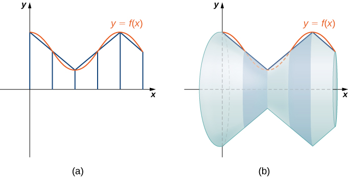
Notice that when each line segment is revolved around the axis, it produces a band. These bands are actually pieces of cones (think of an ice cream cone with the pointy end cut off). A piece of a cone like this is called a frustum of a cone.
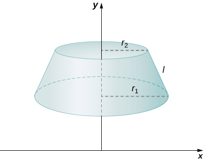
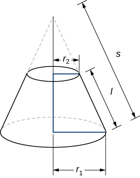
To find the surface area of the band, we need to find the lateral surface area, \(S\), of the frustum (the area of just the slanted outside surface of the frustum, not including the areas of the top or bottom faces). Let \(r_1\) and \(r_2\) be the radii of the wide end and the narrow end of the frustum, respectively, and let \(l\) be the slant height of the frustum as shown in the following figure.
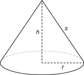
We know the lateral surface area of a cone is given by
\[\text{Lateral Surface Area } =πrs, \nonumber \]
where \(r\) is the radius of the base of the cone and \(s\) is the slant height (Figure \(\PageIndex{7}\)).
Since a frustum can be thought of as a piece of a cone, the lateral surface area of the frustum is given by the lateral surface area of the whole cone less the lateral surface area of the smaller cone (the pointy tip) that was cut off (Figure \(\PageIndex{8}\)).
The cross-sections of the small cone and the large cone are similar triangles, so we see that
\[ \dfrac{r_2}{r_1}=\dfrac{s−l}{s} \nonumber \]
Solving for \(s\), we get =s−ls
\[\begin{align*} \dfrac{r_2}{r_1} &=\dfrac{s−l}{s} \\ r_2s &=r_1(s−l) \\ r_2s &=r_1s−r_1l \\ r_1l &=r_1s−r_2s \\ r_1l &=(r_1−r_2)s \\ \dfrac{r_1l}{r_1−r_2} =s \end{align*}\]
Then the lateral surface area (SA) of the frustum is
\[\begin{align*} S &= \text{(Lateral SA of large cone)}− \text{(Lateral SA of small cone)} \\[4pt] &=πr_1s−πr_2(s−l) \\[4pt] &=πr_1(\dfrac{r_1l}{r_1−r_2})−πr_2(\dfrac{r_1l}{r_1−r_2−l}) \\[4pt] &=\dfrac{πr^2_1l}{r^1−r^2}−\dfrac{πr_1r_2l}{r_1−r_2}+πr_2l \\[4pt] &=\dfrac{πr^2_1l}{r_1−r_2}−\dfrac{πr_1r2_l}{r_1−r_2}+\dfrac{πr_2l(r_1−r_2)}{r_1−r_2} \\[4pt] &=\dfrac{πr^2_1}{lr_1−r_2}−\dfrac{πr_1r_2l}{r_1−r_2} + \dfrac{πr_1r_2l}{r_1−r_2}−\dfrac{πr^2_2l}{r_1−r_3} \\[4pt] &=\dfrac{π(r^2_1−r^2_2)l}{r_1−r_2}=\dfrac{π(r_1−r+2)(r1+r2)l}{r_1−r_2} \\[4pt] &= π(r_1+r_2)l. \label{eq20} \end{align*} \]
Let’s now use this formula to calculate the surface area of each of the bands formed by revolving the line segments around the \(x-axis\). A representative band is shown in the following figure.
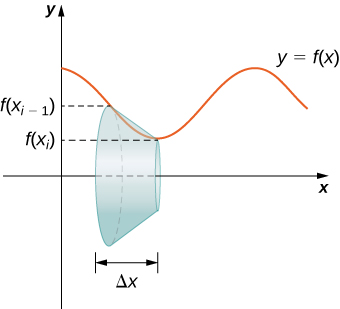
Note that the slant height of this frustum is just the length of the line segment used to generate it. So, applying the surface area formula, we have
\[\begin{align*} S &=π(r_1+r_2)l \\ &=π(f(x_{i−1})+f(x_i))\sqrt{Δx^2+(Δyi)^2} \\ &=π(f(x_{i−1})+f(x_i))Δx\sqrt{1+(\dfrac{Δy_i}{Δx})^2} \end{align*}\]
Now, as we did in the development of the arc length formula, we apply the Mean Value Theorem to select \(x^∗_i∈[x_{i−1},x_i]\) such that \(f′(x^∗_i)=(Δy_i)/Δx.\) This gives us
\[S=π(f(x_{i−1})+f(x_i))Δx\sqrt{1+(f′(x^∗_i))^2} \nonumber \]
Furthermore, since\(f(x)\) is continuous, by the Intermediate Value Theorem, there is a point \(x^{**}_i∈[x_{i−1},x[i]\) such that \(f(x^{**}_i)=(1/2)[f(xi−1)+f(xi)],
so we get
\[S=2πf(x^{**}_i)Δx\sqrt{1+(f′(x^∗_i))^2}.\nonumber \]
Then the approximate surface area of the whole surface of revolution is given by
\[\text{Surface Area} ≈\sum_{i=1}^n2πf(x^{**}_i)Δx\sqrt{1+(f′(x^∗_i))^2}.\nonumber \]
This almost looks like a Riemann sum, except we have functions evaluated at two different points, \(x^∗_i\) and \(x^{**}_{i}\), over the interval \([x_{i−1},x_i]\). Although we do not examine the details here, it turns out that because \(f(x)\) is smooth, if we let n\(→∞\), the limit works the same as a Riemann sum even with the two different evaluation points. This makes sense intuitively. Both \(x^∗_i\) and x^{**}_i\) are in the interval \([x_{i−1},x_i]\), so it makes sense that as \(n→∞\), both \(x^∗_i\) and \(x^{**}_i\) approach \(x\) Those of you who are interested in the details should consult an advanced calculus text.
Taking the limit as \(n→∞,\) we get
\[ \begin{align*} \text{Surface Area} &=\lim_{n→∞}\sum_{i=1}n^2πf(x^{**}_i)Δx\sqrt{1+(f′(x^∗_i))^2} \\[4pt] &=∫^b_a(2πf(x)\sqrt{1+(f′(x))^2}) \end{align*}\]
As with arc length, we can conduct a similar development for functions of \(y\) to get a formula for the surface area of surfaces of revolution about the \(y-axis\). These findings are summarized in the following theorem.
Let \(f(x)\) be a nonnegative smooth function over the interval \([a,b]\). Then, the surface area of the surface of revolution formed by revolving the graph of \(f(x)\) around the x-axis is given by
\[\text{Surface Area}=∫^b_a(2πf(x)\sqrt{1+(f′(x))^2})dx \nonumber \]
Similarly, let \(g(y)\) be a nonnegative smooth function over the interval \([c,d]\). Then, the surface area of the surface of revolution formed by revolving the graph of \(g(y)\) around the \(y-axis\) is given by
\[\text{Surface Area}=∫^d_c(2πg(y)\sqrt{1+(g′(y))^2}dy \nonumber \]
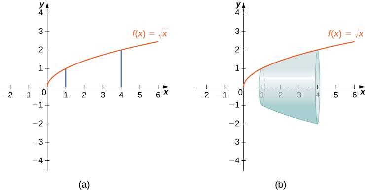
Let \(f(x)=\sqrt{x}\) over the interval \([1,4]\). Find the surface area of the surface generated by revolving the graph of \(f(x)\) around the \(x\)-axis. Round the answer to three decimal places.
Solution
The graph of \(f(x)\) and the surface of rotation are shown in Figure \(\PageIndex{10}\).
We have \(f(x)=\sqrt{x}\). Then, \(f′(x)=1/(2\sqrt{x})\) and \((f′(x))^2=1/(4x).\) Then,
\[\begin{align*} \text{Surface Area} &=∫^b_a(2πf(x)\sqrt{1+(f′(x))^2}dx \\[4pt] &=∫^4_1(\sqrt{2π\sqrt{x}1+\dfrac{1}{4x}})dx \\[4pt] &=∫^4_1(2π\sqrt{x+14}dx. \end{align*}\]
Let \(u=x+1/4.\) Then, \(du=dx\). When \(x=1, u=5/4\), and when \(x=4, u=17/4.\) This gives us
\[\begin{align*} ∫^1_0(2π\sqrt{x+\dfrac{1}{4}})dx &= ∫^{17/4}_{5/4}2π\sqrt{u}du \\[4pt] &= 2π\left[\dfrac{2}{3}u^{3/2}\right]∣^{17/4}_{5/4} \\[4pt] &=\dfrac{π}{6}[17\sqrt{17}−5\sqrt{5}]≈30.846 \end{align*}\]
Let \( f(x)=\sqrt{1−x}\) over the interval \( [0,1/2]\). Find the surface area of the surface generated by revolving the graph of \( f(x)\) around the \(x\)-axis. Round the answer to three decimal places.
- Hint
-
Use the process from the previous example.
- Answer
-
\[ \dfrac{π}{6}(5\sqrt{5}−3\sqrt{3})≈3.133 \nonumber \]
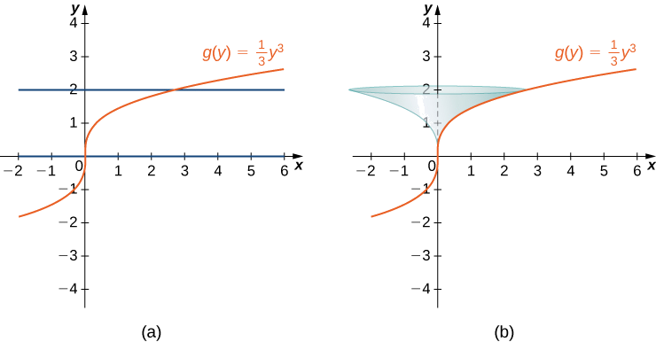
Let \( f(x)=y=\dfrac[3]{3x}\). Consider the portion of the curve where \( 0≤y≤2\). Find the surface area of the surface generated by revolving the graph of \( f(x)\) around the \( y\)-axis.
Solution
Notice that we are revolving the curve around the \( y\)-axis, and the interval is in terms of \( y\), so we want to rewrite the function as a function of \( y\). We get \( x=g(y)=(1/3)y^3\). The graph of \( g(y)\) and the surface of rotation are shown in the following figure.
We have \( g(y)=(1/3)y^3\), so \( g′(y)=y^2\) and \( (g′(y))^2=y^4\). Then
\[\begin{align*} \text{Surface Area} &=∫^d_c(2πg(y)\sqrt{1+(g′(y))^2})dy \\[4pt] &=∫^2_0(2π(\dfrac{1}{3}y^3)\sqrt{1+y^4})dy \\[4pt] &=\dfrac{2π}{3}∫^2_0(y^3\sqrt{1+y^4})dy. \end{align*}\]
Let \( u=y^4+1.\) Then \( du=4y^3dy\). When \( y=0, u=1\), and when \( y=2, u=17.\) Then
\[\begin{align*} \dfrac{2π}{3}∫^2_0(y^3\sqrt{1+y^4})dy &=\dfrac{2π}{3}∫^{17}_1\dfrac{1}{4}\sqrt{u}du \\[4pt] &=\dfrac{π}{6}[\dfrac{2}{3}u^{3/2}]∣^{17}_1=\dfrac{π}{9}[(17)^{3/2}−1]≈24.118. \end{align*}\]
Let \( g(y)=\sqrt{9−y^2}\) over the interval \( y∈[0,2]\). Find the surface area of the surface generated by revolving the graph of \( g(y)\) around the \( y\)-axis.
- Hint
-
Use the process from the previous example.
- Answer
-
\( 12π\)