12.4: Curvature and Normal Vectors of a Curve
( \newcommand{\kernel}{\mathrm{null}\,}\)
For a parametrically defined curve we had the definition of arc length. Since vector valued functions are parametrically defined curves in disguise, we have the same definition. We have the added benefit of notation with vector valued functions in that the square root of the sum of the squares of the derivatives is just the magnitude of the velocity vector.
Let
r(t)=x(t)ˆi+y(t)ˆj+z(t)ˆk
be a differentiable vector valued function on [a,b]. Then the arc length s is defined by
s=∫ba√(dxdt)2+(dydt)2+(dzdt)2dt=∫ba|v(t)|dt.
Suppose that
r(t)=3tˆi+2ˆj+t2ˆk
Set up the integral that defines the arc length of the curve from 2 to 3. Then use a calculator or computer to approximate the arc length.
Solution
We use the arc length formula
s=∫32√9+0+4t2dt=∫32√9+4t2dt.
Notice that we could do this integral by hand by letting t=9/2tanq, however the question only asked us to use a machine to approximate the integral:
s=5.8386.
Parameterization by Arc Length
Recall that like parametric equations, vector valued function describe not just the path of the particle, but also how the particle is moving. Among all representations of a curve there is a "simplest" one. If the particle travels at the constant rate of one unit per second, then we say that the curve is parameterized by arc length. We have seen this concept before in the definition of radians. On a unit circle one radian is one unit of arc length around the circle. When we say "simplest" we in no way mean that the equations are simple to find, but rather that the dynamics of the particle are simple. To aid us in parameterizing by arc length, we define the arc length function.
If r(t) is a differentiable vector valued function, then the arc length function is defined by
s(t)=∫t0||v(u)||du.
Remark: By the second fundamental theorem of calculus, we have
s′(t)=||v(t)||.
If a vector valued function is parameterized by arc length, then
s(t)=t.
If we have a vector valued functionr(t) with arc length s(t), then we can introduce a new variable
s=s−1(t).
So that the vector valued function r(s) will have arc length equal to
s(s−1(t))=t.
and r(s) will be parameterized by arc length. Unfortunately, this process is usually impossible for two reasons.
- The integral that defines arc length involves a square root in the integrand; this integral is usually impossible to determine.
- Even if the integral is possible to evaluate, finding the inverse of a function is often impossible. There are a few special curves that can be parameterized by arc length and one is demonstrated below.
Find the arc length parameterization of the helix defined by
r(t)=costˆi+sintˆj+tˆk.
Solution
First find the arc length function
s(t)=∫t0√sin2u+cos2u+1dt=∫t0√2dt=√2t.
Solving for t gives
t=s√2.
Now substitute back into the position equation to get
r(s)=coss√2ˆi+sins√2ˆj+s√2ˆk.
Concepts: Curvature and Normal Vector
Consider a car driving along a curvy road. The tighter the curve, the more difficult the driving is. In math we have a number, the curvature, that describes this "tightness". If the curvature is zero then the curve looks like a line near this point. While if the curvature is a large number, then the curve has a sharp bend.

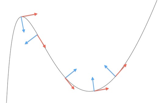
Before learning what curvature of a curve is and how to find the value of that curvature, we must first learn about unit tangent vector. As the name suggests, unit tangent vectors are unit vectors (vectors with length of 1) that are tangent to the curve at certain points. Because tangent lines at certain point of a curve are defined as lines that barely touch the curve at the given point, we can deduce that tangent lines or vectors have slopes equivalent to the instantaneous slope of a curve at the given point. In other words,
T=drdt,
which means
ˆT=T|T|=dr/dt|dr/dt|.
Based on what we learned previosuly, we know that drdt=v, where v is the velocity at which a point is moving at a given time. Furthermore, the absolute value of the velocity vector is the speed vector of the curve, meaning |drdt|=dsdt. So the formula for unit tangent vector can be simplified to:
ˆT=velocityspeed=dr/dtds/dt.
And now, let's think about the unit tangent vector when the curve is explained in terms of arc length, that is, r(s) instead of r(t). This means:
T=drds
and ˆT=dr/dsds/ds=drds.
With this information, we will be learning what curvature really is and how we can calculate the curvature, denoted as κ.
Curvature of a Curve
Curvature is a measure of how much the curve deviates from a straight line. In other words, the curvature of a curve at a point is a measure of how much the change in a curve at a point is changing, meaning the curvature is the magnitude of the second derivative of the curve at given point (let's assume that the curve is defined in terms of the arc length s to make things easier). This means:
k=|d2rds2|.
Since we know that ˆT=dr/ds, we can formulate an equation for κ in terms of ˆT:
k=|dˆTds|.
Never the less, we know that most curves are written in parametric equations in terms of some dummy variable, most commonly t. So let's assume that the curve is in terms of t, such that r(t) is a curve. In such case, we must formulate another equation to find the curvature without taking derivatives in terms of s.
First, we know that
k=|dˆTds|
Using Chain Rule, we get
k=|dˆTdt⋅dtds|=1|ds/dt||dˆTdt|
therefore
k=1|v||dˆTdt|.
Definition of Curvature (repeat)
More formally, if T(t) is the unit tangent vector function then the curvature, k, is defined at the rate at which the unit tangent vector changes with respect to arc length.
k=||dds(T(t))||=||r″(s)||
As stated previously, this is not a practical definition, since parameterizing by arc length is typically impossible. Instead we use the chain rule to get
||dds(T(t))||=||T′(t)dtds||
||T′(t)||||dsdt||=||T′(t)||||r′(t)||.
This formula is more practical to use, but still cumbersome. T′(t) is typically a mess. Instead we can borrow from the formula for the normal vector to get the curvature
K(t)=||r′(t)×r″(t)||||r′(t)||3.
Normal Vector of a Curve
A unit normal vector of a curve, by its definition, is perpendicular to the curve at given point. This means a normal vector of a curve at a given point is perpendicular to the tangent vector at the same point. Furthermore, a normal vector points towards the center of curvature, and the derivative of tangent vector also points towards the center of curvature. In summary, normal vector of a curve is the derivative of tangent vector of a curve.
N=dˆTdsordˆTdt
To find the unit normal vector, we simply divide the normal vector by its magnitude:
ˆN=dˆT/ds|dˆT/ds|ordˆT/dt|dˆT/dt|.
Notice that |dˆT/ds| can be replaced with κ, such that:
ˆN=1κdˆTds
∴
Find the curvature at t=\frac{\pi}{2} if
r(t) = \cos \,t\, \hat{\textbf{i}} - \frac{1}{t} \hat{\textbf{j}} + \sin\, t\, \hat{\textbf{k}} .\nonumber
Solution
We take derivatives
\textbf{r}'(t) = -\sin\, t\, \hat{\textbf{i}} + \frac{1}{t^2}\, \hat{\textbf{j}} + \cos\, t \, \hat{\textbf{k}} \nonumber
\textbf{r}''(t) = -\cos\, t \,\hat{\textbf{i}} - \frac{2}{t^3}\, \hat{\textbf{j}} - \sin\, t\, \hat{\textbf{k}} . \nonumber
Plugging in t=\frac{\pi}{2} gives
\begin{align*} \textbf{r}' \left(\frac{\pi}{2} \right) &= -\hat{\textbf{i}} + \dfrac{4}{\pi^2} \,\hat{\textbf{j}} \\ &= -\dfrac{16}{\pi^3}\, \hat{\textbf{j}} - \hat{\textbf{k}} \end{align*}
\textbf{r}''\left(\frac{\pi}{2}\right) .\nonumber
Now take the cross product to get
\textbf{r}'(\pi/2) \times \textbf{r}''(\pi/2) = -\dfrac{4}{\pi^2} \, \hat{\textbf{i}} -\hat{\textbf{j}} + \dfrac{16}{\pi^3} \, \hat{\textbf{k}} \nonumber
Finally, we plug this information into the curvature formula to get
\dfrac{\sqrt{\dfrac{16}{\pi^4}+1+\dfrac{256}{\pi^6}}}{\left(\sqrt{1+\dfrac{16}{\pi^4}}\right)^3} \approx 0.952 . \nonumber
Curvature of a Plane Curve
If a curve resides only in the xy-plane and is defined by the function y = f(t) then there is an easier formula for the curvature. We can parameterize the curve by
\textbf{r}(t) = t \, \hat{\textbf{i}} + f(t)\, \hat{\textbf{j}} .\nonumber
We have
\textbf{r}'(t) = \hat{\textbf{i}} + f '(t) \, \hat{\textbf{j}} \nonumber
\textbf{r}''(t) = f ''(t) \, \hat{\textbf{j}} .\nonumber
Their cross product is just
r'(t) \times r''(t) = f''(t) \hat{\textbf{k}} \nonumber
which has magnitude
||\textbf{r}'(t) \times r''(t)|| = |f''(t)| . \nonumber
The curvature formula gives
K(t) = \dfrac{|f''(t)|}{ \left[1+\left(f'(t) \right)^2 \right]^{3/2}}. \nonumber
Find the curvature for the curve y = \sin\, x \nonumber .
Solution
We have
f '(x) = \cos \, x \nonumber f ''(x) = -\sin \, x .\nonumber
Plugging into the curvature formula gives K(t) = \dfrac{|-\sin\, t|}{[1+\cos^2t]^{3/2}}\nonumber
The Osculating Circle
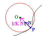
In first year calculus, we saw how to approximate a curve with a line, parabola, etc. Instead we can find the best fitting circle at the point on the curve. If P is a point on the curve, then the best fitting circle will have the same curvature as the curve and will pass through the point P. We will see that the curvature of a circle is a constant 1/r, where r is the radius of the circle. The center of the osculating circle will be on the line containing the normal vector to the circle. In particular the center can be found by adding
OP + 1/K N . \nonumber

The Normal Component of Acceleration Revisited
How is the normal component of acceleration related to the curvature. If you remember, the normal component the acceleration tells us how fast the particle is changing direction. If a curve has a sharp bend (high curvature) then the directional change will be faster. We now show that there is a definite relationship between the normal component of acceleration and curvature.
\textbf{a}(t) = a_{\textbf{T}}\textbf{T}(t) + a_{\textbf{N}}\textbf{N}(t) \nonumber
We have
\begin{align*} \textbf{a}(t) &= \textbf{r}''(t) \\[4pt] &= \dfrac{d}{dt} (\textbf{r}'(t)) \\[4pt] &= \dfrac{d}{dt} \left(||\textbf{r}'(t)||\textbf{T}(t)\right) \\[4pt] &= \dfrac{d}{dt} \left(||r'(t)||)\textbf{T}(t) + ||r'(t)|| \textbf{T}'(t) \right) \\[4pt] &= s''(t)\textbf{T}(t) + s'\textbf{T}'(t) \\[4pt] &= s''(t)\textbf{T}(t) + s'||\textbf{T}'(t)||\textbf{N}(t) = s''(t)\textbf{T}(t) + ks'^2 \textbf{N}(t) .\end{align*}
So that the tangential component of the acceleration is s''(t) and the normal component is k(t)s'^2(t).
Find the tangential and normal components of \textbf{r}(t) = t\, \hat{\textbf{i}}- 2t\, \hat{\textbf{j}} + t^2 \,\hat{\textbf{k}} .
Contributors and Attributions
- Larry Green (Lake Tahoe Community College)
- Joseph Sanghun Lee (UCD)
Integrated by Justin Marshall.

