15.5: Triple Integrals in Rectangular Coordinates
- Page ID
- 2647
\( \newcommand{\vecs}[1]{\overset { \scriptstyle \rightharpoonup} {\mathbf{#1}} } \)
\( \newcommand{\vecd}[1]{\overset{-\!-\!\rightharpoonup}{\vphantom{a}\smash {#1}}} \)
\( \newcommand{\dsum}{\displaystyle\sum\limits} \)
\( \newcommand{\dint}{\displaystyle\int\limits} \)
\( \newcommand{\dlim}{\displaystyle\lim\limits} \)
\( \newcommand{\id}{\mathrm{id}}\) \( \newcommand{\Span}{\mathrm{span}}\)
( \newcommand{\kernel}{\mathrm{null}\,}\) \( \newcommand{\range}{\mathrm{range}\,}\)
\( \newcommand{\RealPart}{\mathrm{Re}}\) \( \newcommand{\ImaginaryPart}{\mathrm{Im}}\)
\( \newcommand{\Argument}{\mathrm{Arg}}\) \( \newcommand{\norm}[1]{\| #1 \|}\)
\( \newcommand{\inner}[2]{\langle #1, #2 \rangle}\)
\( \newcommand{\Span}{\mathrm{span}}\)
\( \newcommand{\id}{\mathrm{id}}\)
\( \newcommand{\Span}{\mathrm{span}}\)
\( \newcommand{\kernel}{\mathrm{null}\,}\)
\( \newcommand{\range}{\mathrm{range}\,}\)
\( \newcommand{\RealPart}{\mathrm{Re}}\)
\( \newcommand{\ImaginaryPart}{\mathrm{Im}}\)
\( \newcommand{\Argument}{\mathrm{Arg}}\)
\( \newcommand{\norm}[1]{\| #1 \|}\)
\( \newcommand{\inner}[2]{\langle #1, #2 \rangle}\)
\( \newcommand{\Span}{\mathrm{span}}\) \( \newcommand{\AA}{\unicode[.8,0]{x212B}}\)
\( \newcommand{\vectorA}[1]{\vec{#1}} % arrow\)
\( \newcommand{\vectorAt}[1]{\vec{\text{#1}}} % arrow\)
\( \newcommand{\vectorB}[1]{\overset { \scriptstyle \rightharpoonup} {\mathbf{#1}} } \)
\( \newcommand{\vectorC}[1]{\textbf{#1}} \)
\( \newcommand{\vectorD}[1]{\overrightarrow{#1}} \)
\( \newcommand{\vectorDt}[1]{\overrightarrow{\text{#1}}} \)
\( \newcommand{\vectE}[1]{\overset{-\!-\!\rightharpoonup}{\vphantom{a}\smash{\mathbf {#1}}}} \)
\( \newcommand{\vecs}[1]{\overset { \scriptstyle \rightharpoonup} {\mathbf{#1}} } \)
\(\newcommand{\longvect}{\overrightarrow}\)
\( \newcommand{\vecd}[1]{\overset{-\!-\!\rightharpoonup}{\vphantom{a}\smash {#1}}} \)
\(\newcommand{\avec}{\mathbf a}\) \(\newcommand{\bvec}{\mathbf b}\) \(\newcommand{\cvec}{\mathbf c}\) \(\newcommand{\dvec}{\mathbf d}\) \(\newcommand{\dtil}{\widetilde{\mathbf d}}\) \(\newcommand{\evec}{\mathbf e}\) \(\newcommand{\fvec}{\mathbf f}\) \(\newcommand{\nvec}{\mathbf n}\) \(\newcommand{\pvec}{\mathbf p}\) \(\newcommand{\qvec}{\mathbf q}\) \(\newcommand{\svec}{\mathbf s}\) \(\newcommand{\tvec}{\mathbf t}\) \(\newcommand{\uvec}{\mathbf u}\) \(\newcommand{\vvec}{\mathbf v}\) \(\newcommand{\wvec}{\mathbf w}\) \(\newcommand{\xvec}{\mathbf x}\) \(\newcommand{\yvec}{\mathbf y}\) \(\newcommand{\zvec}{\mathbf z}\) \(\newcommand{\rvec}{\mathbf r}\) \(\newcommand{\mvec}{\mathbf m}\) \(\newcommand{\zerovec}{\mathbf 0}\) \(\newcommand{\onevec}{\mathbf 1}\) \(\newcommand{\real}{\mathbb R}\) \(\newcommand{\twovec}[2]{\left[\begin{array}{r}#1 \\ #2 \end{array}\right]}\) \(\newcommand{\ctwovec}[2]{\left[\begin{array}{c}#1 \\ #2 \end{array}\right]}\) \(\newcommand{\threevec}[3]{\left[\begin{array}{r}#1 \\ #2 \\ #3 \end{array}\right]}\) \(\newcommand{\cthreevec}[3]{\left[\begin{array}{c}#1 \\ #2 \\ #3 \end{array}\right]}\) \(\newcommand{\fourvec}[4]{\left[\begin{array}{r}#1 \\ #2 \\ #3 \\ #4 \end{array}\right]}\) \(\newcommand{\cfourvec}[4]{\left[\begin{array}{c}#1 \\ #2 \\ #3 \\ #4 \end{array}\right]}\) \(\newcommand{\fivevec}[5]{\left[\begin{array}{r}#1 \\ #2 \\ #3 \\ #4 \\ #5 \\ \end{array}\right]}\) \(\newcommand{\cfivevec}[5]{\left[\begin{array}{c}#1 \\ #2 \\ #3 \\ #4 \\ #5 \\ \end{array}\right]}\) \(\newcommand{\mattwo}[4]{\left[\begin{array}{rr}#1 \amp #2 \\ #3 \amp #4 \\ \end{array}\right]}\) \(\newcommand{\laspan}[1]{\text{Span}\{#1\}}\) \(\newcommand{\bcal}{\cal B}\) \(\newcommand{\ccal}{\cal C}\) \(\newcommand{\scal}{\cal S}\) \(\newcommand{\wcal}{\cal W}\) \(\newcommand{\ecal}{\cal E}\) \(\newcommand{\coords}[2]{\left\{#1\right\}_{#2}}\) \(\newcommand{\gray}[1]{\color{gray}{#1}}\) \(\newcommand{\lgray}[1]{\color{lightgray}{#1}}\) \(\newcommand{\rank}{\operatorname{rank}}\) \(\newcommand{\row}{\text{Row}}\) \(\newcommand{\col}{\text{Col}}\) \(\renewcommand{\row}{\text{Row}}\) \(\newcommand{\nul}{\text{Nul}}\) \(\newcommand{\var}{\text{Var}}\) \(\newcommand{\corr}{\text{corr}}\) \(\newcommand{\len}[1]{\left|#1\right|}\) \(\newcommand{\bbar}{\overline{\bvec}}\) \(\newcommand{\bhat}{\widehat{\bvec}}\) \(\newcommand{\bperp}{\bvec^\perp}\) \(\newcommand{\xhat}{\widehat{\xvec}}\) \(\newcommand{\vhat}{\widehat{\vvec}}\) \(\newcommand{\uhat}{\widehat{\uvec}}\) \(\newcommand{\what}{\widehat{\wvec}}\) \(\newcommand{\Sighat}{\widehat{\Sigma}}\) \(\newcommand{\lt}{<}\) \(\newcommand{\gt}{>}\) \(\newcommand{\amp}{&}\) \(\definecolor{fillinmathshade}{gray}{0.9}\)Just as a single integral has a domain of one-dimension (a line) and a double integral a domain of two-dimension (an area), a triple integral has a domain of three-dimension (a volume). Furthermore, as a single integral produces a value of 2D and a double integral a value of 3D, a triple integral produces a value of higher dimension beyond 3D, namely 4D.
However, because of difficulty in visualizing a four dimensional world, we can simplify and say that a triple integral with a domain of a certain volume, given a function as the density value at a point \((x,y,z)\), produces a value of a mass, which can be written as follows:
\[ \underset{D}{\iiint} \delta (x,y,z) dV \nonumber \]
where \(\delta (x,y,z) \) is the density at point \((x,y,z)\) and because the change in volume equals to the product of change of \(x\), \(y\), and \(z\), it can be rewritten as follows:
\[ \underset{D}{\iiint} \delta (x,y,z) \,dz\, dy\, dx \nonumber \]
in which the order of \(dx\), \(dy\), and \(dz\) does not matter just like the order of \(dx\) and \(dy\) doesn't matter in double integrals.
Triple Integrals in terms of Summation
When we first learned the concept of integrals, we visualized the integral as an area under the curve. However, as we learned more about the integrals, we realized that the integral is a sum of the values at points within a domain, which we divide into infinitely many parts. Likewise, triple integrals can be explained in terms of summation,
\[ \underset{D}{\iiint} f(x,y,z) dV = \underset{n \to \infty} \sum_{i=1}^{n} f(x_{i}, y_{i}, z_{i}) \Delta V_{i}\nonumber \]
where
In another words, we divide the domain into little parts until they become like a point, which appromaxiately has a value of \(f(x,y,z)\). Then we sum up all the values to find the value of the integral.
Volume in terms of Triple Integral
Let's return to the previous visualization of triple integrals as masses given a function of density. Given an object (which is, domain), if we let the density of the object equals to 1, we can assume that the mass of the object equals the volume of the object, because density is mass divided by volume. So if the density = 1, we can use the triple integrals to find the volume, which is also the mass. So,
\[ \mathrm{Volume} = \underset{D}{\iiint} dV.\nonumber \]
In terms of summation, we can visualize the volume of a domain as the sum of all points within the domain. As we have just learned, triple integrals can be viewed as a summation,
\[ \mathrm{Sum } = \underset{n \to \infty}{\lim} \sum_{i=1}^{n} f(x_{i}, y_{i}, z_{i}) \Delta V_{i}\nonumber \]
And if we let \(f(x,y,z) = 1\),
\[ \mathrm{Sum } = \underset{n \to \infty}{\lim} \sum_{i=1}^{n} \Delta V_{i}\nonumber \]
which is simply the sum of all the small cubes, with dimensions \(dx\), \(dy\), \(dz\), in the domain. And as n approaches infinity, the cubes are reduced to dots that fills up the whole domain, which means,
\[ \underset{n \to \infty}{\lim} \sum_{i=1}^{n} \Delta V_{i} = \underset{D}{\iiint} dV\nonumber \]
Average Value of a Function
The average value of a list is defined as the sum of all the values in the list divided by the number of the values in the list. Now when finding the average value of a function \(f(x,y,z)\), we must find the overall sum of all the values of the function within a domain divided by the overall size of the function. In other word,
\[\text{Average Value of } f \approx \dfrac{\sum_{i=1}^{n} f(x_{i},y_{i},z_{i})}{n}\nonumber \]
And before we derive the formula for finding the average value of a function, we must understand that the change in volume, \(dV\), is simply the whole volume within the domain \(D\) divided by some number \(n\).
\[\text{so, } \Delta V = \dfrac{\text{Volume of D}}{n}\nonumber \]
\[\text{which also means, } n = \dfrac{\text{Volume of D}}{\Delta V}\nonumber \]
So using this information we can substitute \(n\) with \(\dfrac{\text{Volume of D}}{dV}\).
\[\text{Average Value of } f \approx \dfrac{\sum_{i=1}^{n} f(x_{i},y_{i},z_{i})}{n}\nonumber \]
\[= \dfrac{\sum_{i=1}^{n} f(x_{i},y_{i},z_{i})}{\dfrac{\text{Volume of D}}{\Delta V}}\nonumber \]
\[= \dfrac{\sum_{i=1}^{n} f(x_{i},y_{i},z_{i}) \Delta V}{\text{Volume of D.}}\nonumber \]
therefore the average value of \(f\) is
\[ \approx \dfrac{1}{\text{Volume of D}} \sum_{i=1}^{n} f(x_{i},y_{i},z_{i}) \Delta V. \nonumber \]
And as \(n\) approaches infinity, meaning dV becomes extremely small, we can find the actual average value of the function.
\[\text{so, Average Value of }f = \dfrac{1}{\text{Volume of D}} \underset{n \to \infty}{\lim} \sum_{i=1}^{n} f(x_{i},y_{i},z_{i}) \Delta V \nonumber \]
\[\therefore \text{Average Value of } f = \dfrac{1}{\text{Volume of D}} \underset{D}{\iiint} f(x,y,z) dV \nonumber \]
Now, from the previous sub-section, we learned that the Volume of \(D\) is the triple integral of the domain \(D\) when \(f(x,y,z) = 1\).
\[\text{So, Average Value of }f = \dfrac{\underset{D}{\iiint} f(x,y,z) dV}{\underset{D}{\iiint} dV.} \nonumber \]
Although the order of integration does not matter in finding the answer, we will be finding the limits of integration in the order of dz, dy, dx just to make the explanation easier. Conceptually, finding the limits is as follows:
- To find the z-limits of integration, we must look at the domain in 3D perspective and draw a ray in the positive z-direction through the center of the domain. Then we must find the lower surface and the upper surface that the ray passes through. And these surfaces are typically expressed in the forms of \(z=f(x,y)\).
- To find the y-limits of integration, we need to look at the domain in 2D perspective, or the x-y surface. So imagine that we have slapped the domain onto the xy-plane, or that we are looking at the domain straight down from the positive z-value. And with the domain in 2D perspective, draw a ray in the positive y-direction through the center of the domain. Then identify two curves, one that the ray passed through first and another later, that are usually expressed in the forms of \(y=f(x)\).
- To find the x-limits of integration, we now need to look at the domain in 1D perspective, or the x-axis. Just like in the case of finding y-limits, let us imagine that we are looking at the 2D domain (note that it is not the original 3D domain but the 2D domain that we were looking at to find the y-limits) from the positive y-value, so that the domain looks like the interval in the x-axis. Then find the lower limit and the upper limit just like how we find the limits in the single integrals.
Find the mass( in kg) of a ball, which has a radius of 2m and a density, \(\mathbf{ \delta (x,y,z) = 2} \) kg / m3.
Solution
We know that the mass can be expressed as an integral of density. \(\text{Meaning, Mass } = \underset{D}{\iiint} \delta (x,y,z) dV\). And we know \( \delta (x,y,z)\) and the domain, which is a sphere with a radius of 2m. So the question is: How do we find the limits of integration if the domain is in the form of \(x^2+y^2+z^2=4\).
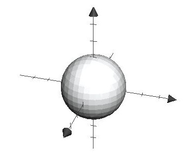
Before finding the z-limits of integration, it is crucial to visualize the domain either through a graph or through a sketch.

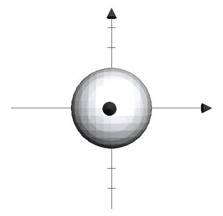
Now to find the z-limits, think of two surfaces, \(z_L=f(x,y)\) and \(z_U=f(x,y)\) that form the domain. With the z-axis as the ray through the center, we can identify that the lower limit is the bottom half of the sphere and the upper limit the top half of the sphere (meaning, the ray enters into the domain from the bottom half first then out through the top half). In other words, \(z_L=-\sqrt{4 - x^2 - y^2}\) and \(z_U=\sqrt{4 - x^2 - y^2}\). Secondly, to find the y-limits, look at the 3D domain from the positive z-value so that the domain looks like a circle as the following:

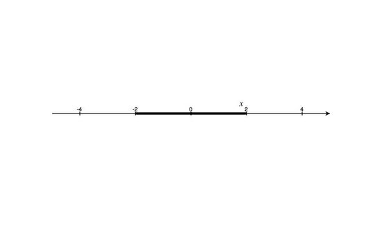
Then, we must find two curves, \(y_L=f(x)\) and \(y_u=f(x)\), that form the circle, \(x^2+y^2=4\). So with the y-axis as the ray through the center of the domain, we can identify the lower limit as the bottom curve of the circle and the upper limit as the top curve of the circle. Therefore, \(y_L=-\sqrt{4-x^2}\) and \(y_U=\sqrt{4-x^2}\). Finally, to find the x-limits, imagine looking at a circular object at its side so that it looks like a line.

Once we view it in a 1D perspective, finding the x-limits is rather simple; it is the interval in the x-axis. In this case, the line stretches from \(x = -2\) to \(x = 2\). So \(x_L=-2\) and \(x_U=2\) (Note that in a definite triple integral, x-limits must be scalar).
Now we must plug in all the information into the triple integral.
\[\begin{align*} \underset{D}{\iiint} \delta (x,y,z) dV &= \int_{x_{L}}^{x_{U}} \int_{y_{L}}^{y_{U}} \int_{z_{L}}^{z_{U}} \delta (x,y,z) \,dz\, dy\, dx \\[4pt] &= \int_{-2}^{2} \int_{-\sqrt{4-x^2}}^{\sqrt{4-x^2}} \int_{-\sqrt{4-x^2-y^2}}^{\sqrt{4-x^2-y^2}} 2 \; dz dy dx \end{align*} \]
However, before we integrate this, we must realize that the density is constant regarless of \(x\), \(y\), or \(z\), and the domain is perfectly symmetric in all \(x\), \(y\), and \(z\) directions. So we can take the integral in the first octant and multiply the result by 8 to obtain the mass. In other words,
\[ \mathrm{Mass } = 8 \int_{0}^{2} \int_{0}^{\sqrt{4-x^2}} \int_{0}^{\sqrt{4-x^2-y^2}} 2 \; dz dy dx. \nonumber \]
And since this integration is rather tedious, we will leave the answer in the integral form.
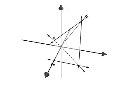
Find the average value of \(\mathbf{f(x,y,z) = 8xyz}\) over a domain bounded by \(\mathbf{z=x+y}\), \(\mathbf{z=0}\), \(\mathbf{y=x}\), \(\mathbf{y=0}\), and \(\mathbf{x=1}\).

Graph of the domain.
First of all, we know that,
\[\textrm{Average Value of }f(x,y,z) = \dfrac{\textrm{Integral of }f(x,y,z) \text{ over D}}{\textrm{Volume of D}}\nonumber \]
So we must find the triple integral of the function \(f(x,y,z)\) and the volume of the domain using the triple integral.
Part 1: Volume
Since calculating the volume is much easier, we will first find the volume of the domain bounded by the planes listed above. And the formula for the volume of domain D is as follows:
\[\text{Volume of D} = \underset{D}{\iiint} dz dy dx.\nonumber \]
In finding the limits of integration, we must notice that the bounds for the domain is rather simple, so we can easily identify the limits:
\[= \int_{0}^{1} \int_{0}^{x} \int_{0}^{x+y} dz dy dx.\nonumber \]
Now, we can simply do the integration as we have learned from double integration.
\[\begin{align*} & = \int_{0}^{1} \int_{0}^{x} \left [ z \right ]_{0}^{x+y} dy dx \nonumber \\[4pt] & = \int_{0}^{1} \int_{0}^{x} x+y dy dx \nonumber \\[4pt] & = \int_{0}^{1} \left [ xy + y^2 \right ]_{0}^{x} dx \nonumber \\[4pt] & = \int_{0}^{1} x^2 + x^2 dx \nonumber \\[4pt] & = \int_{0}^{1} 2x^2 dx \nonumber \\[4pt] & = \left [ \dfrac{2}{3} x^3 \right ]_{0}^{1} \nonumber \\[4pt] & = \dfrac{2}{3} \nonumber \\[4pt] \therefore \textrm{Volume of D} &= \dfrac{2}{3} \end{align*}\nonumber \]
Part 2: Integral of \(f(x,y,z)\) over \(D\)
From what we have learned so far, we know that:
\[ \textrm{Integral of } f(x,y,z) \textrm{over D} = \underset{D}{\iiint} f(x,y,z) dz dy dx. \nonumber \]
And from the part 1, we have already found the limits of integration. So the equation becomes:
\[ = \int_{0}^{1} \int_{0}^{x} \int_{0}^{x+y} 8 x y z \; dz dy dx.\nonumber \]
From this, we can simply do the integration.
\[\begin{align*} & = \int_{0}^{1} \int_{0}^{x} \left [ 4 x y z^2 \right ]_{0}^{x+y} dy dx \nonumber \\[4pt] & = \int_{0}^{1}\int_{0}^{x} 4 x y (x + y)^2 dy dx \nonumber \\[4pt] & = \int_{0}^{1 }\int_{0}^{x} 4xy(x^2+2xy+y^2) dy dx \nonumber \\[4pt] & = \int_{0}^{1 }\int_{0}^{x} 4x^3y + 8x^2y^2 +4xy^3 dy dx \nonumber \\[4pt] & = \int_{0}^{1} \left [ 2x^5 + \dfrac{8}{3}x^2y^3 + xy^4 \right ]_{0}^{x} dx \nonumber \\[4pt] & = \int_{0}^{1} 2x^5 + \dfrac{8}{3}x^5 + x^5 \; dx \nonumber \\[4pt] & = \int_{0}^{1} \dfrac{17}{3} x^5 dx \nonumber \\[4pt] & = \left [ \dfrac{17}{18} x^6 \right ]_{0}^{1} \nonumber \\[4pt] & = \dfrac{17}{18} \nonumber \\[4pt] \therefore \textrm{Integral of } f(x,y,z) &= \dfrac{17}{18} \end{align*}\nonumber \]
Part 3: Average Value of \(f(x,y,z)\)
After calculating the integral of \(f(x,y,z)\) over the domain and the volume of the domain, calculating the average value of the function is extremely esay. As it is stated above,
\[ \textrm{Average Value of } f(x,y,z) = \dfrac{\textrm{Integral of } f(x,y,z)}{\textrm{Volume of D.}}\nonumber \]
Then we substitute the values we found in part 1 and part 2:
\[ \textrm{Average Value of } f(x,y,z) = \dfrac{17/18}{2/3} = \dfrac{17}{12}\nonumber \]
\[\therefore \textrm{Average Value of } f(x,y,z) = \dfrac{17}{12} .\nonumber \]
In a country of slimes, there was a slime king whose massive figure was measured to be 3m wide, 3m long, and 4m tall. After years of research, slime scientists found that the density of a slime is as follows:
\[\mathbf{\delta (x,y,z) = \dfrac{1}{z+1}}. \nonumber \]
However, because the king dislikes complex mathematics involving variables, he ordered the scientists to find the average density of his slime. Using the king's massive figure, calculate the average density of the king.
Solution
First of all, the questions is asking for the average value of the density function. So we must find the volume and the integral of the density function over the domain. Calculating the volume of the slime king is simple:
\[\textrm{Volume} = \textrm{Length x Width x Height}\nonumber \]
\[ = \textrm{3 x 3 x 4} = 36 \textrm{m^3}.\nonumber \]
Now the equation for calculating an average value of a density function is given as follows:
\[\textrm{Integral of } \delta (x,y,z) \textrm{ over D} = \underset{D}{\iiint} \delta (x,y,z) dz dy dx.\nonumber \]
And for this specific problem, it becomes:
\[ = \int_{0}^{3} \int_{0}^{3} \int_{0}^{4} \dfrac{1}{z+1} dz dy dx.\nonumber \]
And from here, it just becomes a simple integration:
\[\begin{align*} & = \int_{0}^{3} \int_{0}^{3} \left [ \ln \left | z+1 \right | \right ]_{0}^{4} dy dx \nonumber \\[4pt] & = \int_{0}^{3} \int_{0}^{3} \ln (5) \; dy dx \nonumber \\[4pt] & = \int_{0}^{3} \left [ \ln (5) y \right ]_{0}^{3}dx \nonumber \\[4pt] & = \int_{0}^{3} 3 \ln (5) dx \nonumber \\[4pt] & = \left [ 3 x \ln (5) \right ]_{0}^{3} \nonumber \\[4pt] &= 9 \ln (5) \textrm{kg.} & \end{align*}\nonumber \]
As for the final answer, we must divide the integral by the volume, to get the average density of the King Slime:
\[ = \dfrac{\textrm{Integral of } \delta}{\textrm{Volume}} = \dfrac{9\ln(5)}{36}\nonumber \]
which is
\[= \dfrac{\ln(5)}{4} \mathrm{kg/m^3}. \nonumber \]
Contributors and Attributions
- Joseph Sanghun Lee (UCD)
Integrated by Justin Marshall.

