
18.5: Explaining the Relations Among Actors in a Network

\newcommand{\vecs}[1]{\overset { \scriptstyle \rightharpoonup} {\mathbf{#1}} }
\newcommand{\vecd}[1]{\overset{-\!-\!\rightharpoonup}{\vphantom{a}\smash {#1}}}
\newcommand{\id}{\mathrm{id}} \newcommand{\Span}{\mathrm{span}}
( \newcommand{\kernel}{\mathrm{null}\,}\) \newcommand{\range}{\mathrm{range}\,}
\newcommand{\RealPart}{\mathrm{Re}} \newcommand{\ImaginaryPart}{\mathrm{Im}}
\newcommand{\Argument}{\mathrm{Arg}} \newcommand{\norm}[1]{\| #1 \|}
\newcommand{\inner}[2]{\langle #1, #2 \rangle}
\newcommand{\Span}{\mathrm{span}}
\newcommand{\id}{\mathrm{id}}
\newcommand{\Span}{\mathrm{span}}
\newcommand{\kernel}{\mathrm{null}\,}
\newcommand{\range}{\mathrm{range}\,}
\newcommand{\RealPart}{\mathrm{Re}}
\newcommand{\ImaginaryPart}{\mathrm{Im}}
\newcommand{\Argument}{\mathrm{Arg}}
\newcommand{\norm}[1]{\| #1 \|}
\newcommand{\inner}[2]{\langle #1, #2 \rangle}
\newcommand{\Span}{\mathrm{span}} \newcommand{\AA}{\unicode[.8,0]{x212B}}
\newcommand{\vectorA}[1]{\vec{#1}} % arrow
\newcommand{\vectorAt}[1]{\vec{\text{#1}}} % arrow
\newcommand{\vectorB}[1]{\overset { \scriptstyle \rightharpoonup} {\mathbf{#1}} }
\newcommand{\vectorC}[1]{\textbf{#1}}
\newcommand{\vectorD}[1]{\overrightarrow{#1}}
\newcommand{\vectorDt}[1]{\overrightarrow{\text{#1}}}
\newcommand{\vectE}[1]{\overset{-\!-\!\rightharpoonup}{\vphantom{a}\smash{\mathbf {#1}}}}
\newcommand{\vecs}[1]{\overset { \scriptstyle \rightharpoonup} {\mathbf{#1}} }
\newcommand{\vecd}[1]{\overset{-\!-\!\rightharpoonup}{\vphantom{a}\smash {#1}}}
\newcommand{\avec}{\mathbf a} \newcommand{\bvec}{\mathbf b} \newcommand{\cvec}{\mathbf c} \newcommand{\dvec}{\mathbf d} \newcommand{\dtil}{\widetilde{\mathbf d}} \newcommand{\evec}{\mathbf e} \newcommand{\fvec}{\mathbf f} \newcommand{\nvec}{\mathbf n} \newcommand{\pvec}{\mathbf p} \newcommand{\qvec}{\mathbf q} \newcommand{\svec}{\mathbf s} \newcommand{\tvec}{\mathbf t} \newcommand{\uvec}{\mathbf u} \newcommand{\vvec}{\mathbf v} \newcommand{\wvec}{\mathbf w} \newcommand{\xvec}{\mathbf x} \newcommand{\yvec}{\mathbf y} \newcommand{\zvec}{\mathbf z} \newcommand{\rvec}{\mathbf r} \newcommand{\mvec}{\mathbf m} \newcommand{\zerovec}{\mathbf 0} \newcommand{\onevec}{\mathbf 1} \newcommand{\real}{\mathbb R} \newcommand{\twovec}[2]{\left[\begin{array}{r}#1 \\ #2 \end{array}\right]} \newcommand{\ctwovec}[2]{\left[\begin{array}{c}#1 \\ #2 \end{array}\right]} \newcommand{\threevec}[3]{\left[\begin{array}{r}#1 \\ #2 \\ #3 \end{array}\right]} \newcommand{\cthreevec}[3]{\left[\begin{array}{c}#1 \\ #2 \\ #3 \end{array}\right]} \newcommand{\fourvec}[4]{\left[\begin{array}{r}#1 \\ #2 \\ #3 \\ #4 \end{array}\right]} \newcommand{\cfourvec}[4]{\left[\begin{array}{c}#1 \\ #2 \\ #3 \\ #4 \end{array}\right]} \newcommand{\fivevec}[5]{\left[\begin{array}{r}#1 \\ #2 \\ #3 \\ #4 \\ #5 \\ \end{array}\right]} \newcommand{\cfivevec}[5]{\left[\begin{array}{c}#1 \\ #2 \\ #3 \\ #4 \\ #5 \\ \end{array}\right]} \newcommand{\mattwo}[4]{\left[\begin{array}{rr}#1 \amp #2 \\ #3 \amp #4 \\ \end{array}\right]} \newcommand{\laspan}[1]{\text{Span}\{#1\}} \newcommand{\bcal}{\cal B} \newcommand{\ccal}{\cal C} \newcommand{\scal}{\cal S} \newcommand{\wcal}{\cal W} \newcommand{\ecal}{\cal E} \newcommand{\coords}[2]{\left\{#1\right\}_{#2}} \newcommand{\gray}[1]{\color{gray}{#1}} \newcommand{\lgray}[1]{\color{lightgray}{#1}} \newcommand{\rank}{\operatorname{rank}} \newcommand{\row}{\text{Row}} \newcommand{\col}{\text{Col}} \renewcommand{\row}{\text{Row}} \newcommand{\nul}{\text{Nul}} \newcommand{\var}{\text{Var}} \newcommand{\corr}{\text{corr}} \newcommand{\len}[1]{\left|#1\right|} \newcommand{\bbar}{\overline{\bvec}} \newcommand{\bhat}{\widehat{\bvec}} \newcommand{\bperp}{\bvec^\perp} \newcommand{\xhat}{\widehat{\xvec}} \newcommand{\vhat}{\widehat{\vvec}} \newcommand{\uhat}{\widehat{\uvec}} \newcommand{\what}{\widehat{\wvec}} \newcommand{\Sighat}{\widehat{\Sigma}} \newcommand{\lt}{<} \newcommand{\gt}{>} \newcommand{\amp}{&} \definecolor{fillinmathshade}{gray}{0.9}In the previous section we looked at some tools for hypotheses about individual actors embedded in networks. Models like these are very useful for examining the relationships among relational and non-relational attributes of individuals.
One of the most distinctive ways in which statistical analysis has been applied to social network data is to focus on predicting the relations of actors, rather than their attributes. Rather than building a statistical model to predict each actor's out-degree, we could, instead, predict whether there was a tie from each actor to each other actor. Rather than explaining the variance in individual persons, we could focus on explaining variation in the relations.
In this final section, we will look at several statistical models that seek to predict the presence or absence (or strength) of a tie between two actors. Models like this are focusing directly on a very sociological question: what factors affect the likelihood that two individuals will have a relationship?
One obvious, but very important, predictor of whether two actors are likely to be connected is their similarity or closeness. In many sociological theories, two actors who share some attribute are predicted to be more likely to form social ties than two actors who do not. This "homophily" hypothesis is at the core of many theories of differentiation, solidarity, and conflict. Two actors who are closer to one in a network are often hypothesized to be more likely to form ties; two actors who share attributes are likely to be at closer distances to one another in networks.
Several of the models below explore homophily and closeness to predict whether actors have ties, or are close to one another. The last model that we will look at the "P1" model also seeks to explain relations. The P1 model tries to predict whether there exists no relation, an asymmetrical relation, or a reciprocated tie between pairs of actors. Rather than using attributes or closeness as predictors, however, the P1 model focuses on basic network properties of each actor and the network as a whole (in-degree, out-degree, global reciprocity). This type of model -- a probability model for the presence/absence of each possible relation in a graph as a function of network structures -- is one of the major continuing areas of development in social network methods.
Hypotheses About Relations Within/Between Groups
One of the most commonplace sociological observations is that "birds of a feather flock together." The notion that similarity (or homophily) increases the probability of the formation of social ties is central to most sociological theories. The homophily hypothesis can be read to be making a prediction about social networks. It suggests that if two actors are similar in some way, it is more likely that there will be network ties between them. If we look at a social network that contains two types of actors, the density of ties ought to be greater within each group than between groups.
Tools>Testing Hypotheses>Mixed Dyadic/Nodal>Categorical Attributes>Joint-Count Provides a test that the density of ties within and between two groups differs from what we would expect if ties were distributed at random across all pairs of nodes.
The procedure takes a binary graph and a partition (that is, a vector that classifies each node as being in one group or the other), and permutes and blocks the data. If there was no association between sharing the same attribute (i.e. being in the same block) and the likelihood of a tie between two actors, we can predict the number of ties that ought to be present in each of the four blocks of the graph (that is: group 1 by group 1; group 1 by group 2; group 2 by group 1; and group 2 by group 2). These four "expected frequencies" can then be compared to the four "observed frequencies." The logic is exactly the same as the Pearson Chi-square test of independence -- we can generate a "test statistic" that shows how far the 2 by 2 table departs from "independence" or "no association."
To test the inferential significance of departures from randomness, however, we cannot rely on standard statistical tables. Instead, a large number of random graphs with the same overall density and the same sized partitions are calculated. The sampling distribution of differences between observed and expected for random graphs can then be calculated, and used to assess the likelihood that our observed graph could be a result of a random trial from a population where there was no association between group membership and the likelihood of a relation.
To illustrate, if two large political donors contributed on the same side of political campaigns (across 48 initiative campaigns), we code them "1" as having a tie or relation, otherwise, we code them zero. We've divided our large political donors in California initiative campaigns into two groups -- those that are affiliated with "workers" (e.g. unions, the Democratic party), and those that are not.
We would anticipate that two groups that represent workers interests would be more likely to share the tie of being in coalitions to support initiatives than would two groups drawn at random. Figure 18.16 shows the results of Tools>Testing Hypotheses>Mixed Dyadic/Nodal>Categorical Attributes>Joint-Count applied to this problem.
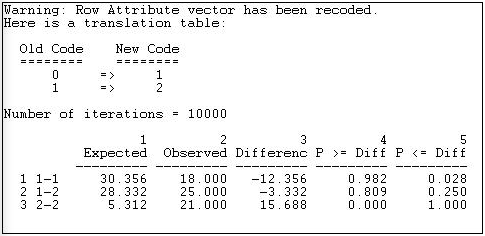
Figure 18.16: Test for two-group differences in tie density
The partition vector (group identification variable) was originally coded as zero for non-worker donors and one for worker donors. These have been re-labeled in the output as one and two. We've used the default of 10,000 random graphs to generate the sampling distribution for group differences.
The first row, labeled "1-1" tells us that, under the null hypothesis that ties are randomly distributed across all actors (i.e. group makes no difference), we would expect 30.356 ties to be present in the non-worker to non-worker block. We actually observe 18 ties in this block, 12 fewer than would be expected. A negative difference this large occurred only 2.8% of the time in graphs where the ties were randomly distributed. It is clear that we have a deviation from randomness within the "non-worker" block. But the difference does not support homophily -- it suggest just the opposite; ties between actors who share the attribute of not representing workers are less likely than random, rather than more likely.
The second row, labeled "1-2" shows no significant difference between the number of ties observed between worker and non-worker groups and what would happen by chance under the null hypothesis of no effect of shared group membership on tie density.
The third row, labeled "2-2" A difference this large indicates that the observed count of ties among interest groups representing workers (21) is much greater than expected by chance (5.3) would almost never be observed if the null hypothesis of no group effect on the probability of ties were true.
Perhaps our result does not support homophily theory because the group "non-worker" is not really as social group at all -- just a residual collection of diverse interests. Using Tools>Testing Hypotheses>Mixed Dyadic/Nodal>Categorical Attributes>Relational Contingency-Table Analysis we can expand the number of groups to provide a better test. This time, let's categorize the political donors as representing "others," "capitalists," or "workers." The results of this test are shown as figure 18.17.
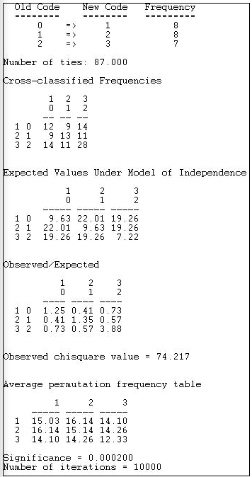
Figure 18.17: Test for three-group differences in tie density
The "other" group has been re-labeled "1," the "capitalist" group re-labeled "2," and the "worker" group re-labeled "3." There are 87 total ties in the graph, with the observed frequencies shown ("Cross-classified Frequencies).
We can see that the the observed frequencies differ from the "Expected Values Under Model of Independence." The magnitudes of the over and under-representation are shown as "Observed/Expected." We note that all three diagonal cells (that is, ties within groups) now display homophily -- greater than random density.
A Pearson chi-square statistic is calculated (74.217). And, we are shown the average tie counts in each cell that occurred in the 10,000 random trials. Finally, we observe that p < 0.0002. That is, the deviation of ties from randomness is so great that it would happen only very rarely if the no-association model was true.
Homophily Models
The result in the section above seems to support homophily (which we can see by looking at where the deviations from independence occur. The statistical test, though, is just a global test of difference from random distribution. The routine Tools>Testing Hypotheses>Mixed Dyadic/Nodal>Categorical Attributes>ANOVA Density Models provides specific tests of some quite specific homophily models.
The least-specific notion of how members of groups relate to members of other groups is simply that the groups differ. Members of one group may prefer to have ties only within their group; members of another group might prefer to have ties only outside of their group.
The Structural Blockmodel option of Tools>Testing Hypotheses>Mixed Dyadic/Nodal>Categorical Attributes>ANOVA Density Models provides a test that the patterns of within and between group ties differ across groups -- but does not specify in what way they may differ. Figure 18.18 shows the results of fitting this model to the data on strong coalition ties (sharing 4 or more campaigns) among "other," "capitalist," and "worker" interest groups.
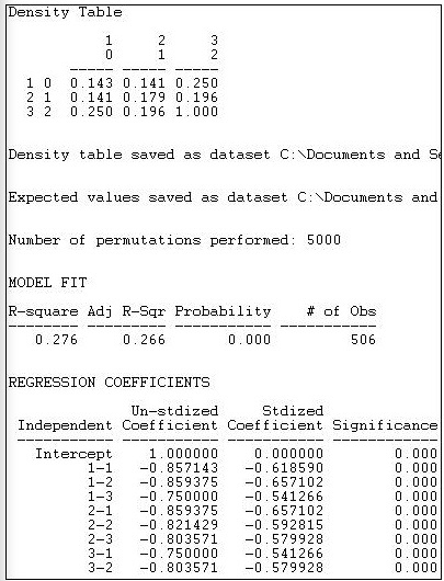
Figure 18.18: Structural block model of differences in group tie density
The observed density table is shown first. Members of the "other" group have a low probability of being tied to one another (0.143) or to "capitalists" (0.143), but somewhat stronger ties to "workers" (0.250). Only the "workers" (category 2, row 3) show strong tendencies toward within-group ties.
Next, a regression model is fit to the data. The presence or absence of a tie between each pair of actors is regressed on a set of dummy variables that represent each of cells of the 3-by-3 table of blocks. In this regression, the last block (i.e. 3-3) is used as the reference category. In our example, the differences among blocks explain 27.6% of the variance in the pair-wise presence or absence of ties. The probability of a tie between two actors, both of whom are in the "workers" block (block 3) is 1.000. The probability in the block describing ties between "other" and "other" actors (block 1-1) is .857 less than this.
The statistical significance of this model cannot be properly assessed using standard formulas for independent observations. Instead, 5000 trials with random permutations of the presence and absence of ties between pairs of actors have been run, and estimated standard errors calculated from the resulting simulated sampling distribution.
A much more restricted notion of group differences is named the Constant Homophily model in Tools>Testing Hypotheses>Mixed Dyadic/Nodal>Categorical Attributes>ANOVA Density Models. This model proposes that all groups may have a preference for within-group ties, but that the strength of the preference is the same within all groups. The results of fitting this model to the data is shown in figure 18.19.
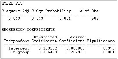
Figure 18.19: Constant Homophily block model of differences in group tie density
Given what we observed in looking directly at the block densities (shown in figure 18.18), it is not surprising that the constant homophily model does not fit these data well. We know that two of the groups ("others" and "capitalists") have no apparent tendency to homophily -- and that differs greatly from the "workers" group. The block model of group differences only accounts for 4.3% of the variance in pair-wise ties; however, permutation trials suggest that this is not a random result (p = 0.001).
This model only has two parameters, because the hypothesis is proposing a simple difference between the diagonal cells (the within group ties 1-1, 2-2, and 3-3) and all other cells. The hypothesis is that the densities within these two partitions are the same. We see that the estimated average tie density of pairs who are not in the same group is 0.193 -- there is a 19.3% chance that heterogeneous dyads will have a tie. If the members of the dyad are from the same group, the probability that they share a tie is 0.196 greater, or 0.389.
So, although the model of constant homophily does not predict individual's ties at all well, there is a notable overall homophily effect.
We noted that the strong tendency toward within-group ties appears to describe only the "workers" group. A third block model, labeled Variable Homophily by Tools>Testing Hypotheses>Mixed Dyadic/Nodal>Categorical Attributes>ANOVA Density Models tests the model that each diagonal cell (that is ties within group 1, within group 2, and within group 3) differ from all ties that are not within-group. Figure 18.20 displays the results.
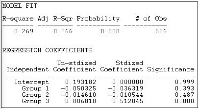
Figure 18.20: Variable homophily block model of differences in group tie density
This model fits the data much better (R-square = 0.269, with p < 0.000) than the constant homophily model. It also fits the data nearly as well as the un-restricted structural block model (Figure 18.18), but is simpler.
Here, the intercept is the probability that there well be a dyadic tie between any two members of different groups (0.193). We see that the probability of within group ties among group 1 ("others") is actually 0.05 less than this (but not significantly different). Within group ties among capitalist interest groups (group 2) are very slightly less common (-0.01) than heterogeneous group ties (again, not significant). Ties among interest groups representing workers (group 3) however, are dramatically more prevalent (0.81) than ties within heterogeneous pairs.
In our example, we noted that one group seems to display in-group ties, and others do not. One way of thinking about this pattern is a "core-periphery" block model. There is a strong form, and a more relaxed form of the core-periphery structure.
The Core-periphery 1 model supposes that there is a highly organized core (many ties within the group), but that there are few other ties -- either among members of the periphery, or between members of the core and members of the periphery. Figure 18.21 shows the results of fitting this block model to the California donors data.
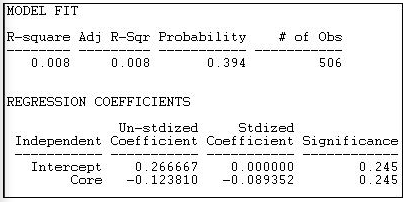
Figure 18.21: "Strong" core-periphery block model of California political donors
It's clear that this model does not do a good job of describing the pattern of within and between group ties. The R-square is very low (0.008), and results this small would occur 39.4% of the time in trials from randomly permuted data. The (non-significant) regression coefficients show density (or the probability of a tie between two random actors) in the periphery as .27, and the density in the "Core" as 0.12 less than this. Since the "core" is, by definition, the maximally dense area, it appears that the output in version 6.8.5 may be mislabeled.
Core-Periphery 2 offers a more relaxed block model in which the core remains densely tied within itself, but is allowed to have ties with the periphery. The periphery is, to the maximum degree possible, a set of cases with no ties within their group. Figure 18.22 shows the results of this model for the California political donors.
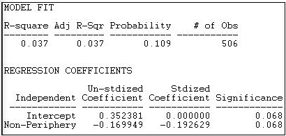
Figure 18.22: "Relaxed" core-periphery block model of California political donors
The fit of this model is better (R-square = 0.037) but still very poor. Results this strong would occur about 11% of the time in trials from randomly permuted data. The intercept density (which we interpret as the "non-periphery") is higher (about 35% of all ties are present), and the probability of a tie between two cases in the periphery is .17 lower.
Hypotheses About Similarity and Distance
The homophily hypothesis is often thought of in categorical terms: is there a tendency for actors who are of the same "type" to be adjacent (or close) to one another in the network?
This idea, though, can be generalized to continuous attributes: is there a tendency for actors who have more similar attributes to be located closer to one another in a network?
UCINET's Tools>Testing Hypotheses>Mixed Dyadic?Nodal>Continuous Attributes>Moran/Geary statistics provides two measures that address the question of the "autocorrelation" between actor's scores on interval-level measures of their attributes, and the network distance between them. The two measures (Moran's I and Geary's C) are adapted for social network analysis from their origins in geography, where they were developed to measure the extent to which the similarity of the geographical features of any two places was related to the spatial distance between them.
Let's suppose that we were interested in whether there was a tendency for political interest groups that were "close" to one another to spend similar amounts of money. We might suppose that interest groups that are frequent allies may also influence one another in terms of the levels of resources they contribute -- that a sort of norm of expected levels of contribution arises among frequent allies.
Using information about the contributions of very large donors (who gave over a total of $5,000,000) to at least four (of 48) ballot initiatives in California, we can illustrate the idea of network autocorrelation.
First, we create an attribute file that contains a column that has the attribute score of each node, in this case, the amount of total expenditures by the donors.
Second, we create a matrix data set that describes the "closeness" of each pair of actors. There are several alternative approaches here. One is to use an adjacency (binary) matrix. We will illustrate this by coding two donors as adjacent if they contributed funds on the same side of at least four campaigns (here, we've constructed adjacency from "affiliation" data; often we have a direct measure of adjacency, such as one donor naming another as an ally). We could also use a continuous measure of the strength of the tie between actors as a measure of "closeness." To illustrate this, we will use a scale of the similarity of the contribution profiles of donors that ranges from negative numbers (indicating that two donors gave money on opposite sides of initiatives) to positive numbers (indicating the number of times the donated on the same side of issues. One can easily imagine other approaches to indexing the network closeness of actors (e.g. 1/geodesic distance). Any "proximity" matrix that captures the pair-wise closeness of actors can be used (for some ideas, see Tools>Similarities and Tools>Dissimilarities and Distances).
Figures 18.23 and 18.24 display the results of Tools>Testing Hypotheses>Mixed Dyadic/Nodal>Continuous Attributes>Moran/Geary statistics where we have examined the autocorrelation of the levels of expenditures of actors using adjacency as our measure of network distance. Very simply: do actors who are adjacent in the network tend to give similar amounts of money? Two statistics and some related information are presented (the Moran statistic in Figure 18.23, and the Geary statistic in Figure 18.24.
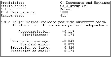
Figure 18.23: Moran autocorrelation of expenditure levels by political donors with network adjacency
The Moran "I" statistic of autocorrelation (originally developed to measure spatial autocorrelation, but used here to measure network autocorrelation) ranges from -1.0 (perfect negative correlation) through 0 (no correlation) to +1.0 (perfect positive correlation). Here we see the value of -0.119, indicating that there is a very modest tendency for actors who are adjacent to differ more in how much they contribute than two random actors. If anything, it appears that coalition members may vary more in their contribution levels than random actors -- another hypothesis bites the dust!
The Moran statistic (see any geo-statistics text, or do a Google search) is constructed very much like a regular correlation coefficient. It indexes the product of the differences between the scores of two actors and the mean, weighted by the actor's similarity - that is, a covariance weighted by the closeness of actors. This sum is taken in ratio to variance in the scores of all actors from the mean. The resulting measure, like the correlation coefficient, is a ratio of covariance to variance, and has a conventional interpretation.
Permutation trials are used to create a sampling distribution. Across many (in our example 1,000) trials, scores on the attribute (expenditure, in this case) are randomly assigned to actors, and the Moran statistic calculated. In these random trials, the average observed Moran statistic is -0.043, with a standard deviation of .073. The difference between what we observe (-0.119) and what is predicted by random association (-0.043) is small relative to sampling variability. In fact, 17.4% of all samples from random data showed correlations at least this big -- far more than the conventional 5% acceptable error rate.
The Geary measure of correlation is calculated and interpreted somewhat differently. Results are shown in Figure 18.24 for the association of expenditure levels by network adjacency.

Figure 18.24: Geary autocorrelation of expenditure levels by political donors with network adjacency
The Geary statistic has a value of 1.0 when there is no association. Values less than 1.0 indicate a positive association (somewhat confusingly), values greater than 1.0 indicate a negative association. Our calculated value of 2.137 indicates negative autocorrelation, just as the Moran statistic did. Unlike the Moran statistic though, the Geary statistic suggests that the difference of our result from the average of 1,000 random trials (1.004) is statistically significant (p = 0.026).
The Geary statistic is sometimes described in the geo-statistics literature as being more sensitive to "local" differences than to "global" differences. The Geary C statistic is constructed by examining the differences between the scores of each pair of actors, and weighting this by their adjacency. The Moran statistic is constructed by looking at differences between each actor's score and the mean, and weighting the cross-products. The difference in approach means that the Geary statistic is more focused on how different members of each pair are from each other - a "local" difference; the Moran statistic is focused more on how the similar or dissimilar each pair are to the overall average -- a "global" difference.
In data where the "landscape" of values displays a lot of variation, and non-normal distribution, the two measures are likely to give somewhat different impressions about the effects of network adjacency on similarity of attributes. As always, it's not that one is "right" and the other "wrong." It's always best to compute both, unless you have strong theoretical priors that suggest that one is superior for a particular purpose.
Figures 18.25 and 18.26 repeat the exercise above, but with one difference. In these two examples, we measure the closeness of two actors in the network on a continuous scale. Here, we've used the net number of campaigns on which each pair of actors were in the same coalition as a measure of closeness. Other measures, like geodesic distances might be more commonly used for true network data (rather than a network inferred from affiliation).
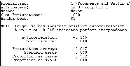
Figure 18.25: Moran autocorrelation of expenditure levels by political donors with network closeness
Using a continuous measure of network closeness (instead of adjacency) we might expect a stronger correlation. The Moran measure is now -0.145 ( compared to -0.119), and is significant at p = 0.018. There is a small, but significant tendency for actors who are "close" allies to give different amounts of money than two randomly chosen actors -- a negative network autocorrelation.
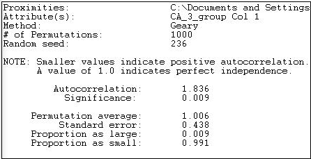
Figure 18.26: Geary autocorrelation of expenditure levels by political donors with network closeness
The Geary measure has become slightly smaller in size (1.836 versus 2.137) using a continuous measure of network distance. The result also indicates a negative autocorrelation, and one that would rarely occur by chance if there truly was no association between network distance and expenditure.
The Probability of a Dyadic Tie: Leinhardt's P1
The approaches that we've been examining in this section look at the relationship between actor's attributes and their location in a network. Before closing our discussion of how statistical analysis has been applied to network data, we need to look at one approach that examines how ties between pairs of actors relate to particularly important relational attributes of the actors, and to a more global feature of the graph.
For any pair of actors in a directed graph, there are three possible relationships: no ties, an asymmetric tie, or a reciprocated tie. Network>P1 is a regression-like approach that seeks to predict the probability of each of these kinds of relationships for each pair of actors. This differs a bit from the approaches that we've examined so far which seek to predict either the presence/absence of a tie, or the strength of a tie.
The P1 model (and its newer successor the P* model), seek to predict the dyadic relations among actor pairs using key relational attributes of each actor, and of the graph as a whole. This differs from most of the approaches that we've seen above, which focus on actor's individual or relational attributes, but do not include overall structural features of the graph (at least not explicitly).
The P1 model consists of three prediction equations, designed to predict the probability of a mutual (i.e. reciprocated) relation (mij), an asymmetric relation (aij), or a null relation (nij) between actors. The equations, as stated by the authors of UCINET are:
m_{ij} = \lambda_{ij} e^{\rho + 2 \theta + \alpha_i + \alpha_j + \hat{a}_i + \hat{a}_j}
a_{ij} = \lambda_{ij} e^{\theta + \alpha_i + \beta_j}
n_{ij} = \lambda_{ij}
The first equation says that the probability of a reciprocated tie between two actors is a function of the out-degree (or "expansiveness") of each actor: alphai and alphaj. It is also a function of the overall density of the network (theta). It is also a function of the global tendency in the whole network toward reciprocity (rho). The equation also contains scaling constants for each actor in the pair (ai and aj), as well as a global scaling parameter (lambda).
The second equation describes the probability that two actors will be connected with an asymmetric relation. This probability is a function of the overall network density (theta), and the propensity of one actor of the pair to send ties (expansiveness, or alpha), and the propensity of the other actor to receive ties ("attractiveness" or beta).
The probability of a null relation (no tie) between two actors is a "residual." That is, if ties are not mutual or asymmetric, they must be null. Only the scaling constant "lambda," and no causal parameters enter the third equation.
The core idea here is that we try to understand the relations between pairs of actors as functions of individual relational attributes (individual's tendencies to send ties, and to receive them) as well as key features of the graph in which the two actors are embedded (the overall density and overall tendency towards reciprocity). More recent versions of the model (P*, P2) include additional global features of the graph such as tendencies toward transitivity and the variance across actors in the propensity to send and receive ties.
Figure 18.27 shows the results of fitting the P1 model to the Knoke binary information network.
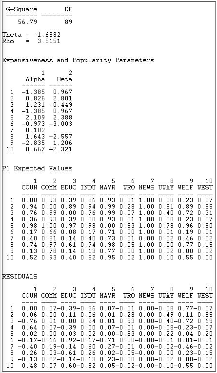
Figure 18.27: Results of P1 analysis of Knoke information network
The technical aspects of the estimation of the P1 model are complicated, and maximum likelihood methods are used. A G-square (likelihood ratio chi-square) badness of fit statistic is provided, but has no direct interpretation or significance test.
Two descriptive parameters for global network properties are given:
- \theta = -1.6882 refers to the effect of the global density of the network on the probability of reciprocated or asymmetric ties between pairs of actors.
- \rho = 3.5151 refers to the effect of the overall amount of reciprocity in the global network on the probability of a reciprocated tie between any pair of actors.
Two descriptive parameters are given for each actor (these are estimated across all of the pair-wise relations of each actor):
\alpha ("expansiveness") refers to the effect of each actor's out-degree on the probability that they will have reciprocated or asymmetric ties with other actors. We see, for example, that the Mayor (actor 5) is a relatively "expansive" actor.
\beta ("attractiveness") refers to the effect of each actor's in-degree on the probability that they will have a reciprocated or asymmetric relation with other actors. We see here, for example, that the welfare rights organization (actor 6) is very likely to be shunned.
Using the equations, it is possible to predict the probability of each directed tie based on the model's parameters. These are shown as the "P1 expected values." For example, the model predicts a 93% chance of a tie from actor 1 to actor 2.
The final panel of the output shows the difference between the ties that actually exist, and the predictions of the model. The model predicts the tie from actor 1 to actor 2 quite well (residual = .07), but it does a poor job of predicting the relation from actor 1 to actor 9 (residual = 0.77).
The residuals important because they suggest places where other features of the graph or individuals may be relevant to understanding particular dyads, or where the ties between two actors is well accounted for by basic "demographics" of the network. Which actors are likely to have ties that are not predicted by the parameters of the model can also be shown in a dendogram, as in Figure 18.28.
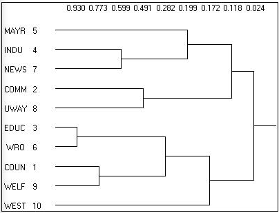
Figure 18.28: Diagram of P1 clustering of Knoke information network
Here we see that, for example, that actors 3 and 6 are much more likely to have ties than the P1 model predicts.