9.5: Calculus and Polar Functions

The previous section defined polar coordinates, leading to polar functions. We investigated plotting these functions and solving a fundamental question about their graphs, namely, where do two polar graphs intersect?

We now turn our attention to answering other questions, whose solutions require the use of calculus. A basis for much of what is done in this section is the ability to turn a polar function $r=f(\theta)$ into a set of parametric equations. Using the identities $x=r\cos \theta$ and $y=r\sin \theta$, we can create the parametric equations $x=f(\theta)\cos\theta$, $y=f(\theta)\sin\theta$ and apply the concepts of Section 9.3.

Polar Functions and $\frac{dy}{dx}$

We are interested in the lines tangent a given graph, regardless of whether that graph is produced by rectangular, parametric, or polar equations. In each of these contexts, the slope of the tangent line is $\frac{dy}{dx}$. Given $r=f(\theta)$, we are generally not concerned with $r^\prime =f^\prime (\theta)$; that describes how fast $r$ changes with respect to $\theta$. Instead, we will use $x=f(\theta)\cos\theta$, $y=f(\theta)\sin\theta$ to compute $\frac{dy}{dx}$.

Using Key Idea 37 we have $$\frac{dy}{dx} = \frac{dy}{d\theta}\Big/\frac{dx}{d\theta}.$$

Each of the two derivatives on the right hand side of the equality requires the use of the Product Rule. We state the important result as a Key Idea.

key idea 41 Finding $\frac{dy}{dx}$ with Polar Functions

Let $r=f(\theta)$ be a polar function. With $x=f(\theta)\cos\theta$ and $y=f(\theta)\sin\theta$,

$$\frac{dy}{dx} = \frac{f^\prime (\theta)\sin\theta+f(\theta)\cos\theta}{f^\prime (\theta)\cos\theta-f(\theta)\sin\theta}.$$

Example $\PageIndex{1}$: Finding $\frac{dy}{dx}$ with polar functions.

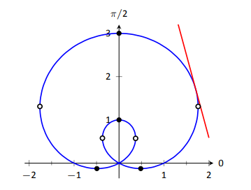
Consider the limacon $r=1+2\sin\theta$ on $[0,2\pi]$.

1. Find the equations of the tangent and normal lines to the graph at $\theta=\pi/4$.
2. Find where the graph has vertical and horizontal tangent lines.

Solution

1. We start by computing $\frac{dy}{dx}$. With $f^\prime (\theta) = 2\cos\theta$, we have $$\begin{align*}\frac{dy}{dx} &= \frac{2\cos\theta\sin\theta + \cos\theta(1+2\sin\theta)}{2\cos^2\theta-\sin\theta(1+2\sin\theta)}\\&= \frac{\cos\theta(4\sin\theta+1)}{2(\cos^2\theta-\sin^2\theta)-\sin\theta}.\end{align*}$$
   
   When $\theta=\pi/4$, $\frac{dy}{dx}=-2\sqrt{2}-1$ (this requires a bit of simplification). In rectangular coordinates, the point on the graph at $\theta=\pi/4$ is $(1+\sqrt{2}/2,1+\sqrt{2}/2)$. Thus the rectangular equation of the line tangent to the limacon at $\theta=\pi/4$ is $$y=(-2\sqrt{2}-1)\big(x-(1+\sqrt{2}/2)\big)+1+\sqrt{2}/2 \approx -3.83 x+8.24.$$ The limacon and the tangent line are graphed in Figure 9.47.
   The normal line has the opposite--reciprocal slope as the tangent line, so its equation is
   $$y \approx \frac{1}{3.83}x+1.26.$$
   
2. To find the horizontal lines of tangency, we find where $\frac{dy}{dx}=0$; thus we find where the numerator of our equation for $\frac{dy}{dx}$ is 0.
   $$\cos\theta(4\sin\theta+1)=0\quad \Rightarrow \quad \cos\theta=0 \quad \text{or}\quad 4\sin\theta+1=0.$$
   On $[0,2\pi]$, $\cos\theta=0$ when $\theta=\pi/2,\ 3\pi/2$.
   
   Setting $4\sin\theta+1=0$ gives $\theta=\sin^{-1}(-1/4)\approx -0.2527 = -14.48^\circ$. We want the results in $[0,2\pi]$; we also recognize there are two solutions, one in the 3$^\text{rd}$ quadrant and one in the 4$^\text{th}$. Using reference angles, we have our two solutions as $\theta =3.39$ and $6.03$ radians. The four points we obtained where the limacon has a horizontal tangent line are given in Figure 9.47 with black--filled dots.
   
   To find the vertical lines of tangency, we set the denominator of $\frac{dy}{dx}=0$.
   $$\begin{align*}2(\cos^2\theta -\sin^2\theta)-\sin\theta &= 0 .\\ \text{Convert the \(\cos^2\theta\) term to \(1-\sin^2\theta\):}& \\ 2(1-\sin^2\theta-\sin^2\theta)-\sin\theta &= 0\\4\sin^2\theta + \sin\theta -1 &= 0.\\ \text{Recognize this as a quadratic in the variable \(\sin\theta\).}&\text{ Using the quadratic formula, we have} \\\sin\theta &= \frac{-1\pm\sqrt{33}}{8}.\end{align*}$$
   
   We solve $\sin\theta = \frac{-1+\sqrt{33}}8$ and $\sin\theta = \frac{-1-\sqrt{33}}8$:
   $$\begin{align*}\sin\theta &=\frac{-1+\sqrt{33}}8 & \sin\theta &= \frac{-1-\sqrt{33}}{8}\\\theta &= \sin^{-1}\left(\frac{-1+\sqrt{33}}8\right) & \theta &= \sin^{-1}\left(\frac{-1-\sqrt{33}}8\right)\\ \theta &= 0.6399 & \theta &= -1.0030\end{align*}$$
   
   In each of the solutions above, we only get one of the possible two solutions as $\sin^{-1}x$ only returns solutions in $[-\pi/2,\pi/2]$, the 4$^\text{th}$ and $1^\text{st}$ quadrants. Again using reference angles, we have:
   $$\sin\theta = \frac{-1+\sqrt{33}}8 \quad \Rightarrow \quad \theta = 0.6399,\ 3.7815 \text{ radians}$$
   and
   $$\sin\theta = \frac{-1-\sqrt{33}}8 \quad \Rightarrow \quad \theta = 4.1446,\ 5.2802 \text{ radians.}$$
   These points are also shown in Figure 9.47 with white--filled dots.

Figure 9.47: The limacon in Example 9.5.1 with its tangent line at $\theta = \pi /4$ and points of vertical and horizontal tangency.

When the graph of the polar function $r=f(\theta)$ intersects the pole, it means that $f(\alpha)=0$ for some angle $\alpha$. Thus the formula for $\frac{dy}{dx}$ in such instances is very simple, reducing simply to

$$\frac{dy}{dx} = \tan \alpha.$$

This equation makes an interesting point. It tells us the slope of the tangent line at the pole is $\tan \alpha$; some of our previous work (see, for instance, Example 9.4.3) shows us that the line through the pole with slope $\tan \alpha$ has polar equation $\theta=\alpha$. Thus when a polar graph touches the pole at $\theta=\alpha$, the equation of the tangent line at the pole is $\theta=\alpha$.

Example $\PageIndex{2}$: Finding tangent lines at the pole.

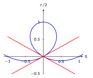
Let $r=1+2\sin\theta$, a limacon. Find the equations of the lines tangent to the graph at the pole.

Figure 9.48: Graphing the tangent lines at the pole in Example 9.5.2.

Solution

We need to know when $r=0$.

$$\begin{align*} 1+2\sin\theta &= 0\\ \sin\theta &= -1/2\\ \theta &= \frac{7\pi}{6},\ \frac{11\pi}6. \end{align*}$$

Thus the equations of the tangent lines, in polar, are $\theta = 7\pi/6$ and $\theta = 11\pi/6$. In rectangular form, the tangent lines are $y=\tan(7\pi/6)x$ and $y=\tan(11\pi/6)x$. The full limacon con can be seen in Figure 9.47; we zoom in on the tangent lines in Figure 9.48.

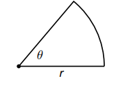
Note: Recall that the area of a sector of a circle with radius r subtended by an angle $\theta$ is $A=\frac{1}{2}\theta r^2$.

Area

When using rectangular coordinates, the equations $x=h$ and $y=k$ defined vertical and horizontal lines, respectively, and combinations of these lines create rectangles (hence the name "rectangular coordinates''). It is then somewhat natural to use rectangles to approximate area as we did when learning about the definite integral.

When using polar coordinates, the equations $\theta=\alpha$ and $r=c$ form lines through the origin and circles centered at the origin, respectively, and combinations of these curves form sectors of circles. It is then somewhat natural to calculate the area of regions defined by polar functions by first approximating with sectors of circles.

Consider Figure 9.49 (a) where a region defined by $r=f(\theta)$ on $[\alpha,\beta]$ is given. (Note how the "sides'' of the region are the lines $\theta=\alpha$ and $\theta=\beta$, whereas in rectangular coordinates the "sides'' of regions were often the vertical lines $x=a$ and $x=b$.)

Figure 9.49: Computing the area of a polar region.

Partition the interval $[\alpha,\beta]$ into $n$ equally spaced subintervals as $\alpha = \theta_1 < \theta_2 <\cdots <\theta_{n+1}=\beta$. The length of each subinterval is $\Delta\theta = (\beta-\alpha)/n$, representing a small change in angle. The area of the region defined by the $i\,^\text{th}$ subinterval $[\theta_i,\theta_{i+1}]$ can be approximated with a sector of a circle with radius $f(c_i)$, for some $c_i$ in $[\theta_i,\theta_{i+1}]$. The area of this sector is $\frac12f(c_i)^2\Delta\theta$. This is shown in part (b) of the figure, where $[\alpha,\beta]$ has been divided into 4 subintervals. We approximate the area of the whole region by summing the areas of all sectors:

$$\text{Area} \approx \sum_{i=1}^n \frac12f(c_i)^2\Delta\theta.$$

This is a Riemann sum. By taking the limit of the sum as $n\to\infty$, we find the exact area of the region in the form of a definite integral.

THEOREM 83 AREA OF A POLAR REGION

Let $f$ be continuous and non-negative on $[\alpha,\beta]$, where $0\leq \beta-\alpha\leq 2\pi$. The area $A$ of the region bounded by the curve $r=f(\theta)$ and the lines $\theta=\alpha$ and $\theta=\beta$ is

$$A \ =\ \frac12\int_\alpha^\beta f(\theta)^2 \ d\theta\ =\ \frac12\int_\alpha^\beta r^{\,2} \ d\theta$$

The theorem states that $0\leq \beta-\alpha\leq 2\pi$. This ensures that region does not overlap itself, which would give a result that does not correspond directly to the area.

Example $\PageIndex{3}$: Area of a polar region

Find the area of the circle defined by $r=\cos \theta$. (Recall this circle has radius $1/2$.)

Solution

This is a direct application of Theorem 83. The circle is traced out on $[0,\pi]$, leading to the integral

$$\begin{align*} \text{Area} &= \frac12\int_0^\pi \cos^2\theta\ d \theta \\ &= \frac12\int_0^\pi \frac{1+\cos(2\theta)}{2}\ d\theta\\ &= \frac14\big(\theta +\frac12\sin(2\theta)\big)\Bigg|_0^\pi\\ &= \frac14\pi. \end{align*}$$

Of course, we already knew the area of a circle with radius $1/2$. We did this example to demonstrate that the area formula is correct.

Note: Example 9.5.3 requires the use of the integral $\int \cos^2\theta\ d\theta$. This is handled well by using the power reducing formula as found in the back of this text. Due to the nature of the area formula, integrating $\cos^2\theta$ and $\sin^2\theta$ is required often. We offer here these indefinite integrals as a time--saving measure.

$$\int\cos^2\theta\ d\theta = \frac12\theta+\frac14\sin(2\theta)+C$$

$$\int\sin^2\theta\ d\theta = \frac12\theta-\frac14\sin(2\theta)+C$$

Example $\PageIndex{4}$: Area of a polar region

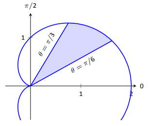
Find the area of the cardiod $r=1+\cos\theta$ bound between $\theta=\pi/6$ and $\theta=\pi/3$, as shown in Figure 9.50.

Figure 9.50: Finding the area of the shaded region of a cardiod in Example 9.5.4

Solution
This is again a direct application of Theorem 83.

$$\begin{align*} \text{Area} &= \frac12\int_{\pi/6}^{\pi/3} (1+\cos\theta)^2\ d\theta\\ &= \frac12\int_{\pi/6}^{\pi/3} (1+2\cos\theta+\cos^2\theta)\ d\theta\\ &= \frac12\left(\theta+2\sin\theta+\frac12\theta+\frac14\sin(2\theta)\right)\Bigg|_{\pi/6}^{\pi/3} \\ &= \frac18\big(\pi+4\sqrt{3}-4\big) \approx 0.7587. \end{align*}$$

Area Between Curves

Our study of area in the context of rectangular functions led naturally to finding area bounded between curves. We consider the same in the context of polar functions. \index{polar!functions!area between curves}

Consider the shaded region shown in Figure 9.51. We can find the area of this region by computing the area bounded by $r_2=f_2(\theta)$ and subtracting the area bounded by $r_1=f_1(\theta)$ on $[\alpha,\beta]$. Thus

$$\text{Area}\ = \ \frac12\int_\alpha^\beta r_2^{\,2}\ d\theta - \frac12\int_\alpha^\beta r_1^{\,2}\ d\theta = \frac12\int_\alpha^\beta \big(r_2^{\,2}-r_1^{\,2}\big)\ d\theta.$$

Figure 9.51: Illustrating area bound between two polar curves.

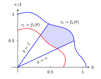
KEY IDEA 42 area between polar curves

The area $A$ of the region bounded by $r_1=f_1(\theta)$ and $r_2=f_2(\theta)$, $\theta=\alpha$ and $\theta=\beta$, where $f_1(\theta)\leq f_2(\theta)$ on $[\alpha,\beta]$, is

$$A = \frac12\int_\alpha^\beta \big(r_2^{\,2}-r_1^{\,2}\big)\ d\theta.$$

Example $\PageIndex{5}$: Area between polar curves

Find the area bounded between the curves $r=1+\cos \theta$ and $r=3\cos\theta$, as shown in Figure 9.52.

Figure 9.52: Finding the area between polar curves in Example 9.5.5.

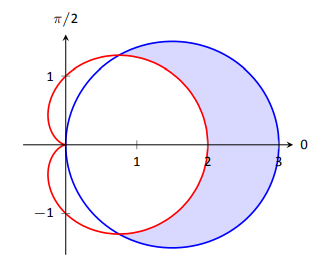
Solution
We need to find the points of intersection between these two functions. Setting them equal to each other, we find:

$$\begin{align*} 1+\cos\theta &= 3\cos \theta \\ \cos\theta &=1/2\\ \theta &= \pm \pi/3 \end{align*}$$

Thus we integrate $\frac12\big((3\cos\theta)^2-(1+\cos\theta)^2\big)$ on $[-\pi/3,\pi/3]$.

$$\begin{align*} \text{Area} &= \frac12\int_{-\pi/3}^{\pi/3} \big((3\cos\theta)^2-(1+\cos\theta)^2\big)\ d\theta\\ &= \frac12\int_{-\pi/3}^{\pi/3} \big( 8\cos^2\theta-2\cos\theta-1\big)\ d\theta \\ &= \big(2\sin(2\theta) - 2\sin\theta+3\theta\big)\Bigg|_{-\pi/3}^{\pi/3}\\ &= 2\pi. \end{align*}$$

Amazingly enough, the area between these curves has a "nice'' value

Example $\PageIndex{6}$: Area defined by polar curves

Find the area bounded between the polar curves $r=1$ and $r=2\cos(2\theta)$, as shown in Figure 9.53 (a).

Solution

We need to find the point of intersection between the two curves. Setting the two functions equal to each other, we have

$$2\cos(2\theta) = 1 \quad \Rightarrow \quad \cos(2\theta) = \frac12 \quad \Rightarrow \quad 2\theta = \pi/3\quad \Rightarrow \quad \theta=\pi/6.$$

Figure 9.53: Graphing the region bounded by the functions in Example 9.5.6

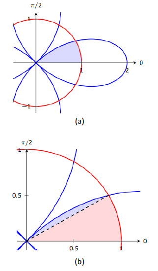
In part (b) of the figure, we zoom in on the region and note that it is not really bounded between two polar curves, but rather by two polar curves, along with $\theta=0$. The dashed line breaks the region into its component parts. Below the dashed line, the region is defined by $r=1$, $\theta=0$ and $\theta = \pi/6$. (Note: the dashed line lies on the line $\theta=\pi/6$.) Above the dashed line the region is bounded by $r=2\cos(2\theta)$ and $\theta =\pi/6$. Since we have two separate regions, we find the area using two separate integrals.

Call the area below the dashed line $A_1$ and the area above the dashed line $A_2$. They are determined by the following integrals:
$$A_1 = \frac12\int_0^{\pi/6} (1)^2\ d\theta\qquad A_2 = \frac12\int_{\pi/6}^{\pi/4} \big(2\cos(2\theta)\big)^2\ d\theta.$$
(The upper bound of the integral computing $A_2$ is $\pi/4$ as $r=2\cos(2\theta)$ is at the pole when $\theta=\pi/4$.)

We omit the integration details and let the reader verify that $A_1 = \pi/12$ and $A_2 = \pi/12-\sqrt{3}/8$; the total area is $A = \pi/6-\sqrt{3}/8$.

Arc Length

As we have already considered the arc length of curves defined by rectangular and parametric equations, we now consider it in the context of polar equations. Recall that the arc length $L$ of the graph defined by the parametric equations $x=f(t)$, $y=g(t)$ on $[a,b]$ is

$$L = \int_a^b \sqrt{f^\prime (t)^2 + g^\prime(t)^2}\ dt = \int_a^b \sqrt{x^\prime(t)^2+y^\prime (t)^2}\ dt.\label{eq:polar_arclength}$$

Now consider the polar function $r=f(\theta)$. We again use the identities $x=f(\theta)\cos\theta$ and $y=f(\theta)\sin\theta$ to create parametric equations based on the polar function. We compute $x^\prime(\theta)$ and $y^\prime (\theta)$ as done before when computing $\frac{dy}{dx}$, then apply Equation $\ref{eq:polar_arclength}$.

The expression $x^\prime(\theta)^2+y^\prime (\theta)^2$ can be simplified a great deal; we leave this as an exercise and state that $$x^\prime(\theta)^2+y^\prime (\theta)^2 = f^\prime (\theta)^2+f(\theta)^2.$$
This leads us to the arc length formula.

key idea 43 arc length of polar curves

Let $r=f(\theta)$ be a polar function with $f^\prime$ continuous on an open interval $I$ containing $[\alpha,\beta]$, on which the graph traces itself only once. The arc length $L$ of the graph on $[\alpha,\beta]$ is
$$L = \int_\alpha^\beta \sqrt{f^\prime (\theta)^2+f(\theta)^2}\ d\theta = \int_\alpha^\beta\sqrt{(r^\prime )^2+ r^2}\ d\theta.$$

Example $\PageIndex{7}$: Arc length of a limacon

Find the arc length of the limacon $r=1+2\sin t$.

Solution

With $r=1+2\sin t$, we have $r^\prime = 2\cos t$. The limacon is traced out once on $[0,2\pi]$, giving us our bounds of integration. Applying Key Idea 43, we have

$$\begin{align*} L &= \int_0^{2\pi} \sqrt{(2\cos\theta)^2+(1+2\sin\theta)^2}\ d\theta \\ &= \int_0^{2\pi} \sqrt{4\cos^2\theta+4\sin^2\theta +4\sin\theta+1}\ d\theta\\ &= \int_0^{2\pi} \sqrt{4\sin\theta+5}\ d\theta\\ &\approx 13.3649. \end{align*}$$

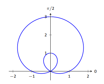
Figure 9.54: The limacon in Example 9.5.7 whose arc length is measured.

The final integral cannot be solved in terms of elementary functions, so we resorted to a numerical approximation. (Simpson's Rule, with $n=4$, approximates the value with $13.0608$. Using $n=22$ gives the value above, which is accurate to 4 places after the decimal.)

Surface Area

The formula for arc length leads us to a formula for surface area. The following Key Idea is based on Key Idea 39.

KEY IDEA 44 SURFACE AREA OF A SOLID OF REVOLUTION

Consider the graph of the polar equation $r=f(\theta)$, where $f^\prime$ is continuous on an open interval containing $[\alpha,\beta]$ on which the graph does not cross itself.

1. The surface area of the solid formed by revolving the graph about the initial ray ($\theta=0$) is: $$\text{Surface Area} = 2\pi\int_\alpha^\beta f(\theta)\sin\theta\sqrt{f^\prime (\theta)^2+f(\theta)^2}\ d\theta.$$
2. The surface area of the solid formed by revolving the graph about the line $\theta=\pi/2$ is: $$\text{Surface Area} = 2\pi\int_\alpha^\beta f(\theta)\cos\theta\sqrt{f^\prime (\theta)^2+f(\theta)^2}\ d\theta.$$

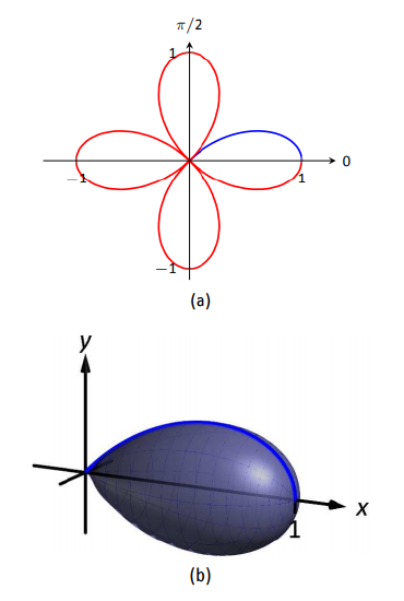
Example $\PageIndex{8}$: Surface area determined by a polar curve

Find the surface area formed by revolving one petal of the rose curve $r=\cos(2\theta)$ about its central axis (see Figure 9.55.

Solution

We choose, as implied by the figure, to revolve the portion of the curve that lies on $[0,\pi/4]$ about the initial ray. Using Key Idea $\ref{idea:surface_area_polar}$ and the fact that $f^\prime (\theta) = -2\sin(2\theta)$, we have

$$\begin{align*} \text{Surface Area} &= 2\pi\int_0^{\pi/4} \cos(2\theta)\sin(\theta)\sqrt{\big(-2\sin(2\theta)\big)^2+\big(\cos(2\theta)\big)^2}\ d\theta \\ &\approx 1.36707. \end{align*}$$

The integral is another that cannot be evaluated in terms of elementary functions. Simpson's Rule, with $n=4$, approximates the value at $1.36751$.%; with $n=10$, the value is accurate to 4 decimal places.

Figure 9.55: Finding the surface area of a rose-curve petal that is revolved around its central axis.

This chapter has been about curves in the plane. While there is great mathematics to be discovered in the two dimensions of a plane, we live in a three dimensional world and hence we should also look to do mathematics in 3D -- that is, in space. The next chapter begins our exploration into space by introducing the topic of vectors, which are incredibly useful and powerful mathematical objects.

Contributors and Attributions

• Gregory Hartman (Virginia Military Institute). Contributions were made by Troy Siemers and Dimplekumar Chalishajar of VMI and Brian Heinold of Mount Saint Mary's University. This content is copyrighted by a Creative Commons Attribution - Noncommercial (BY-NC) License. http://www.apexcalculus.com/