
4.4: Differentials
- Page ID
- 4174

\( \newcommand{\vecs}[1]{\overset { \scriptstyle \rightharpoonup} {\mathbf{#1}} } \)
\( \newcommand{\vecd}[1]{\overset{-\!-\!\rightharpoonup}{\vphantom{a}\smash {#1}}} \)
\( \newcommand{\dsum}{\displaystyle\sum\limits} \)
\( \newcommand{\dint}{\displaystyle\int\limits} \)
\( \newcommand{\dlim}{\displaystyle\lim\limits} \)
\( \newcommand{\id}{\mathrm{id}}\) \( \newcommand{\Span}{\mathrm{span}}\)
( \newcommand{\kernel}{\mathrm{null}\,}\) \( \newcommand{\range}{\mathrm{range}\,}\)
\( \newcommand{\RealPart}{\mathrm{Re}}\) \( \newcommand{\ImaginaryPart}{\mathrm{Im}}\)
\( \newcommand{\Argument}{\mathrm{Arg}}\) \( \newcommand{\norm}[1]{\| #1 \|}\)
\( \newcommand{\inner}[2]{\langle #1, #2 \rangle}\)
\( \newcommand{\Span}{\mathrm{span}}\)
\( \newcommand{\id}{\mathrm{id}}\)
\( \newcommand{\Span}{\mathrm{span}}\)
\( \newcommand{\kernel}{\mathrm{null}\,}\)
\( \newcommand{\range}{\mathrm{range}\,}\)
\( \newcommand{\RealPart}{\mathrm{Re}}\)
\( \newcommand{\ImaginaryPart}{\mathrm{Im}}\)
\( \newcommand{\Argument}{\mathrm{Arg}}\)
\( \newcommand{\norm}[1]{\| #1 \|}\)
\( \newcommand{\inner}[2]{\langle #1, #2 \rangle}\)
\( \newcommand{\Span}{\mathrm{span}}\) \( \newcommand{\AA}{\unicode[.8,0]{x212B}}\)
\( \newcommand{\vectorA}[1]{\vec{#1}} % arrow\)
\( \newcommand{\vectorAt}[1]{\vec{\text{#1}}} % arrow\)
\( \newcommand{\vectorB}[1]{\overset { \scriptstyle \rightharpoonup} {\mathbf{#1}} } \)
\( \newcommand{\vectorC}[1]{\textbf{#1}} \)
\( \newcommand{\vectorD}[1]{\overrightarrow{#1}} \)
\( \newcommand{\vectorDt}[1]{\overrightarrow{\text{#1}}} \)
\( \newcommand{\vectE}[1]{\overset{-\!-\!\rightharpoonup}{\vphantom{a}\smash{\mathbf {#1}}}} \)
\( \newcommand{\vecs}[1]{\overset { \scriptstyle \rightharpoonup} {\mathbf{#1}} } \)
\(\newcommand{\longvect}{\overrightarrow}\)
\( \newcommand{\vecd}[1]{\overset{-\!-\!\rightharpoonup}{\vphantom{a}\smash {#1}}} \)
\(\newcommand{\avec}{\mathbf a}\) \(\newcommand{\bvec}{\mathbf b}\) \(\newcommand{\cvec}{\mathbf c}\) \(\newcommand{\dvec}{\mathbf d}\) \(\newcommand{\dtil}{\widetilde{\mathbf d}}\) \(\newcommand{\evec}{\mathbf e}\) \(\newcommand{\fvec}{\mathbf f}\) \(\newcommand{\nvec}{\mathbf n}\) \(\newcommand{\pvec}{\mathbf p}\) \(\newcommand{\qvec}{\mathbf q}\) \(\newcommand{\svec}{\mathbf s}\) \(\newcommand{\tvec}{\mathbf t}\) \(\newcommand{\uvec}{\mathbf u}\) \(\newcommand{\vvec}{\mathbf v}\) \(\newcommand{\wvec}{\mathbf w}\) \(\newcommand{\xvec}{\mathbf x}\) \(\newcommand{\yvec}{\mathbf y}\) \(\newcommand{\zvec}{\mathbf z}\) \(\newcommand{\rvec}{\mathbf r}\) \(\newcommand{\mvec}{\mathbf m}\) \(\newcommand{\zerovec}{\mathbf 0}\) \(\newcommand{\onevec}{\mathbf 1}\) \(\newcommand{\real}{\mathbb R}\) \(\newcommand{\twovec}[2]{\left[\begin{array}{r}#1 \\ #2 \end{array}\right]}\) \(\newcommand{\ctwovec}[2]{\left[\begin{array}{c}#1 \\ #2 \end{array}\right]}\) \(\newcommand{\threevec}[3]{\left[\begin{array}{r}#1 \\ #2 \\ #3 \end{array}\right]}\) \(\newcommand{\cthreevec}[3]{\left[\begin{array}{c}#1 \\ #2 \\ #3 \end{array}\right]}\) \(\newcommand{\fourvec}[4]{\left[\begin{array}{r}#1 \\ #2 \\ #3 \\ #4 \end{array}\right]}\) \(\newcommand{\cfourvec}[4]{\left[\begin{array}{c}#1 \\ #2 \\ #3 \\ #4 \end{array}\right]}\) \(\newcommand{\fivevec}[5]{\left[\begin{array}{r}#1 \\ #2 \\ #3 \\ #4 \\ #5 \\ \end{array}\right]}\) \(\newcommand{\cfivevec}[5]{\left[\begin{array}{c}#1 \\ #2 \\ #3 \\ #4 \\ #5 \\ \end{array}\right]}\) \(\newcommand{\mattwo}[4]{\left[\begin{array}{rr}#1 \amp #2 \\ #3 \amp #4 \\ \end{array}\right]}\) \(\newcommand{\laspan}[1]{\text{Span}\{#1\}}\) \(\newcommand{\bcal}{\cal B}\) \(\newcommand{\ccal}{\cal C}\) \(\newcommand{\scal}{\cal S}\) \(\newcommand{\wcal}{\cal W}\) \(\newcommand{\ecal}{\cal E}\) \(\newcommand{\coords}[2]{\left\{#1\right\}_{#2}}\) \(\newcommand{\gray}[1]{\color{gray}{#1}}\) \(\newcommand{\lgray}[1]{\color{lightgray}{#1}}\) \(\newcommand{\rank}{\operatorname{rank}}\) \(\newcommand{\row}{\text{Row}}\) \(\newcommand{\col}{\text{Col}}\) \(\renewcommand{\row}{\text{Row}}\) \(\newcommand{\nul}{\text{Nul}}\) \(\newcommand{\var}{\text{Var}}\) \(\newcommand{\corr}{\text{corr}}\) \(\newcommand{\len}[1]{\left|#1\right|}\) \(\newcommand{\bbar}{\overline{\bvec}}\) \(\newcommand{\bhat}{\widehat{\bvec}}\) \(\newcommand{\bperp}{\bvec^\perp}\) \(\newcommand{\xhat}{\widehat{\xvec}}\) \(\newcommand{\vhat}{\widehat{\vvec}}\) \(\newcommand{\uhat}{\widehat{\uvec}}\) \(\newcommand{\what}{\widehat{\wvec}}\) \(\newcommand{\Sighat}{\widehat{\Sigma}}\) \(\newcommand{\lt}{<}\) \(\newcommand{\gt}{>}\) \(\newcommand{\amp}{&}\) \(\definecolor{fillinmathshade}{gray}{0.9}\)In Section 2.2 we explored the meaning and use of the derivative. This section starts by revisiting some of those ideas.
Recall that the derivative of a function \(f\) can be used to find the slopes of lines tangent to the graph of \(f\). At \(x=c\), the tangent line to the graph of \(f\) has equation
$$y = f'(c)(x-c)+f(c).\]
The tangent line can be used to find good approximations of \(f(x)\) for values of \(x\) near \(c\).
For instance, we can approximate \(\sin 1.1\) using the tangent line to the graph of \(f(x)=\sin x\) at \(x=\pi/3 \approx 1.05.\) Recall that \(\sin (\pi/3) = \sqrt{3}/2 \approx 0.866\), and \(\cos (\pi/3) = 1/2\). Thus the tangent line to \(f(x) = \sin x\) at \(x=\pi/3\) is:
$$ \ell(x) = \frac12(x-\pi/3)+0.866.\]
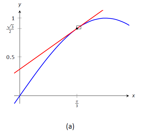
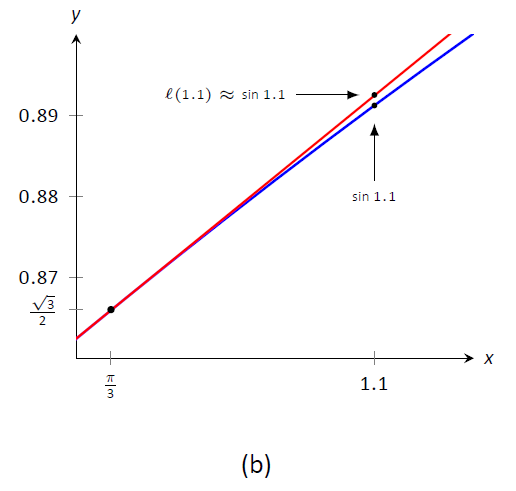
Figure \(\PageIndex{1}\): Graphing \(f(x) = \sin x\) and its tangent line at \(x=\pi/3\) in order to estimate \(\sin 1.1\).
In Figure \(\PageIndex{1a}\), we see a graph of \(f(x) = \sin x\) graphed along with its tangent line at \(x=\pi/3\). The small rectangle shows the region that is displayed in Figure \(\PageIndex{1b}\). In this figure, we see how we are approximating \(\sin 1.1\) with the tangent line, evaluated at \(1.1\). Together, the two figures show how close these values are.
Using this line to approximate \(\sin 1.1\), we have:
\[ \begin{align} \ell(1.1) &= \frac12(1.1-\pi/3)+0.866 \\ &= \frac12(0.053)+0.866 = 0.8925. \end{align}\]
(We leave it to the reader to see how good of an approximation this is.)
We now generalize this concept. Given \(f(x)\) and an \(x\)--value \(c\), the tangent line is \(\ell(x) = f'(c)(x-c)+f(c)\). Clearly, \(f(c) = \ell(c)\). Let \(\Delta x\) be a small number, representing a small change in \(x\) value. We assert that:
$$f(c+\Delta x) \approx \ell(c+\Delta x),\]
since the tangent line to a function approximates well the values of that function near \(x=c\).
As the \(x\) value changes from \(c\) to \(c+\Delta x\), the \(y\) value of \(f\) changes from \(f(c)\) to \(f(c+\Delta x)\). We call this change of \(y\) value \(\Delta y\). That is:
$$\Delta y = f(c+\Delta x)-f(c).\]
Replacing \(f(c+\Delta x)\) with its tangent line approximation, we have
\[ \begin{align} \Delta y &\approx \ell(c+\Delta x) - f(c) \notag\\ &= f'(c)\big((c+\Delta x)-c\big)+f(c) - f(c)\notag \\ &=f'(c)\Delta x \end{align}\]
This final equation is important; we'll come back to it in Key Idea 7.
We introduce two new variables, \(dx\) and \(dy\) in the context of a formal definition.
Definition: Differentials of \(x\) and \(y\).
Let \(y=f(x)\) be differentiable. The differential of \(x\), denoted \(dx\), is any nonzero real number (usually taken to be a small number). The differential of \(y\), denoted \(dy\), is
\[dy = f'(x)dx.\]
We can solve for \(f'(x)\) in the above equation: \(f'(x) = dy/dx\). This states that the derivative of \(f\) with respect to \(x\) is the differential of \(y\) divided by the differential of \(x\); this is not the alternate notation for the derivative, \(\frac{dy}{dx}\). This latter notation was chosen because of the fraction--like qualities of the derivative, but again, it is one symbol and not a fraction.
It is helpful to organize our new concepts and notations in one place.
Key Idea 7: Differential Notation
Let \(y = f(x)\) be a differentiable function.
- \(\Delta x\) represents a small, nonzero change in \(x\) value.
- \(dx\) represents a small, nonzero change in \(x\) value (i.e., \(\Delta x = dx\)).
- \(\Delta y\) is the change in \(y\) value as \(x\) changes by \(\Delta x\); hence $$\Delta y = f(x+\Delta x)-f(x).$$
- \(dy = f'(x)dx\) which, by Equation \(\PageIndex{7}\), is an approximation of the change in \(y\) value as \(x\) changes by \(\Delta x\); \(dy \approx \Delta y\).
What is the value of differentials? Like many mathematical concepts, differentials provide both practical and theoretical benefits. We explore both here.
Example \(\PageIndex{1}\): Finding and using differentials
Consider \(f(x) = x^2\). Knowing \(f(3) = 9\), approximate \(f(3.1)\).
Solution
The \(x\) value is changing from \(x=3\) to \(x=3.1\); therefore, we see that \(dx=0.1\). If we know how much the \(y\) value changes from \(f(3)\) to \(f(3.1)\) (i.e., if we know \(\Delta y\)), we will know exactly what \(f(3.1)\) is (since we already know \(f(3)\)). We can approximate \Delta y\ with \(dy\).
\[ \begin{align} \Delta y &\approx dy \\ &= f'(3)dx \\ &= 2\cdot 3\cdot 0.1 = 0.6. \end{align}\]
We expect the \(y\) value to change by about \(0.6\), so we approximate \(f(3.1) \approx 9.6.\)
We leave it to the reader to verify this, but the preceding discussion links the differential to the tangent line of \(f(x)\) at \(x=3\). One can verify that the tangent line, evaluated at \(x=3.1\), also gives \(y=9.6\).
Of course, it is easy to compute the actual answer (by hand or with a calculator): \(3.1^2 = 9.61.\) (Before we get too cynical and say "Then why bother?", note our approximation is really good!)
So why bother?
In "most" real life situations, we do not know the function that describes a particular behavior. Instead, we can only take measurements of how things change -- measurements of the derivative.
Imagine water flowing down a winding channel. It is easy to measure the speed and direction (i.e., the velocity) of water at any location. It is very hard to create a function that describes the overall flow, hence it is hard to predict where a floating object placed at the beginning of the channel will end up. However, we can approximate the path of an object using differentials. Over small intervals, the path taken by a floating object is essentially linear. Differentials allow us to approximate the true path by piecing together lots of short, linear paths. This technique is called Euler's Method, studied in introductory Differential Equations courses.
We use differentials once more to approximate the value of a function. Even though calculators are very accessible, it is neat to see how these techniques can sometimes be used to easily compute something that looks rather hard.
Example \(\PageIndex{2}\): Using differentials to approximate a function value
Approximate \(\sqrt{4.5}\).
Solution
We expect \(\sqrt{4.5} \approx 2\), yet we can do better. Let \(f(x) = \sqrt{x}\), and let \(c=4\). Thus \(f(4) = 2\). We can compute \(f'(x) = 1/(2\sqrt{x})\), so \(f'(4) = 1/4\).
We approximate the difference between \(f(4.5)\) and \(f(4)\) using differentials, with \(dx = 0.5\):
$$f(4.5)-f(4) = \Delta y \approx dy = f'(4)\cdot dx = 1/4 \cdot 1/2 = 1/8 = 0.125.\]
The approximate change in \(f\) from \(x=4\) to \(x=4.5\) is \(0.125\), so we approximate \(\sqrt{4.5} \approx 2.125.\)
Differentials are important when we discuss integration. When we study that topic, we will use notation such as
$$\int f(x)\ dx\]
quite often. While we don't discuss here what all of that notation means, note the existence of the differential \(dx\). Proper handling of integrals comes with proper handling of differentials.
In light of that, we practice finding differentials in general.
Example \(\PageIndex{3}\): Finding differentials
In each of the following, find the differential \(dy\).
\[y = \sin x \qquad\quad 2. y = e^x(x^2+2) \quad\qquad 3. y = \sqrt{x^2+3x-1}\]
Solution
- \(y = \sin x\): As \(f(x) = \sin x\), \(f'(x) = \cos x\). Thus $$dy = \cos (x)dx.$$
- \(y = e^x(x^2+2)\): Let \(f(x) = e^x(x^2+2)\). We need \(f'(x)\), requiring the Product Rule.
We have \(f'(x) = e^x(x^2+2) + 2xe^x\), so $$dy = \big(e^x(x^2+2) + 2xe^x\big)dx.$$ - \(y = \sqrt{x^2+3x-1}\): Let \(f(x) = \sqrt{x^2+3x-1}\); we need \(f'(x)\), requiring the Chain Rule.
We have \(\Delta s f'(x) = \frac{1}{2}(x^2+3x-1)^{-\frac12}(2x+3) = \frac{2x+3}{2\sqrt{x^2+3x-1}}.\) Thus $$dy = \frac{(2x+3)dx}{2\sqrt{x^2+3x-1}}.$$
Finding the differential \(dy\) of \(y=f(x)\) is really no harder than finding the derivative of \(f\); we just multiply \(f'(x)\) by \(dx\). It is important to remember that we are not simply adding the symbol "\(dx\)" at the end.
We have seen a practical use of differentials as they offer a good method of making certain approximations. Another use is error propagation. Suppose a length is measured to be \(x\), although the actual value is \(x+\Delta x\) (where we hope \Delta x\ is small). This measurement of \(x\) may be used to compute some other value; we can think of this as \(f(x)\) for some function \(f\). As the true length is \(x+\Delta x\), one really should have computed \(f(x+\Delta x)\). The difference between \(f(x)\) and \(f(x+\Delta x)\) is the propagated error.
How close are \(f(x)\) and \(f(x+\Delta x)\)? This is a difference in "y" values;
$$f(x+\Delta x)-f(x) = \Delta y \approx dy.\]
We can approximate the propagated error using differentials.
Example \(\PageIndex{4}\): Using differentials to approximate propagated error
A steel ball bearing is to be manufactured with a diameter of 2cm. The manufacturing process has a tolerance of \(\pm 0.1\)mm in the diameter. Given that the density of steel is about 7.85g/cm\(^3\), estimate the propagated error in the mass of the ball bearing.
Solution
The mass of a ball bearing is found using the equation "mass = volume \(\times\) density." In this situation the mass function is a product of the radius of the ball bearing, hence it is \(m = 7.85\frac43\pi r^3\). The differential of the mass is
$$dm = 31.4\pi r^2 dr.\]
The radius is to be 1cm; the manufacturing tolerance in the radius is \(\pm 0.05\)mm, or \(\pm 0.005\)cm. The propagated error is approximately:
\[\begin{align} \Delta m & \approx dm \\ &= 31.4\pi (1)^2 (\pm 0.005) \\ &= \pm 0.493\text{g} \end{align}\]
Is this error significant? It certainly depends on the application, but we can get an idea by computing the relative error. The ratio between amount of error to the total mass is
\[\begin{align} \frac{dm}{m} &= \pm \frac{0.493}{7.85\frac43\pi} \\ &=\pm \frac{0.493}{32.88}\\ &=\pm 0.015,\end{align}\]
or \(\pm 1.5\).
We leave it to the reader to confirm this, but if the diameter of the ball was supposed to be 10cm, the same manufacturing tolerance would give a propagated error in mass of \(\pm12.33\)g, which corresponds to a \textit{percent error} of \(\pm0.188\)\%. While the amount of error is much greater ($12.33 > 0.493$), the percent error is much lower.
We first learned of the derivative in the context of instantaneous rates of change and slopes of tangent lines. We furthered our understanding of the power of the derivative by studying how it relates to the graph of a function (leading to ideas of increasing/decreasing and concavity). This chapter has put the derivative to yet more uses:
- Equation solving (Newton's Method)
- Related Rates (furthering our use of the derivative to find instantaneous rates of change)
- Optimization (applied extreme values), and
- Differentials (useful for various approximations and for something called integration).
In the next chapters, we will consider the "reverse" problem to computing the derivative: given a function \(f\), can we find a function whose derivative is \(f\)? Be able to do so opens up an incredible world of mathematics and applications.
Contributors and Attributions
Gregory Hartman (Virginia Military Institute). Contributions were made by Troy Siemers and Dimplekumar Chalishajar of VMI and Brian Heinold of Mount Saint Mary's University. This content is copyrighted by a Creative Commons Attribution - Noncommercial (BY-NC) License. http://www.apexcalculus.com/
Integrated by Justin Marshall.