2.5: Maxima and Minima

- Last updated
- Jan 16, 2023
- Save as PDF

( \newcommand{\kernel}{\mathrm{null}\,}\)
The gradient can be used to find extreme points of real-valued functions of several variables, that is, points where the function has a local maximum or local minimum. We will consider only functions of two variables; functions of three or more variables require methods using linear algebra.
Definition 2.7
Let f(x,y) be a real-valued function, and let (a,b) be a point in the domain of f. We say that f has a local maximum at (a,b) if f(x,y)≤f(a,b) for all (x,y) inside some disk of positive radius centered at (a,b), i.e. there is some sufficiently small r>0 such that f(x,y)≤f(a,b) for all (x,y) for which (x−a)2+(y−b)2<r2.
Likewise, we say that f has a local minimum at (a,b) if f(x,y)>f(a,b) for all (x,y) inside some disk of positive radius centered at (a,b).
If f(x,y)≤f(a,b) for all (x,y) in the domain of f, then f has a global maximum at (a,b). If f(x,y)≥f(a,b) for all (x,y) in the domain of f, then f has a global minimum at (a,b).
Suppose that (a,b) is a local maximum point for f(x,y), and that the first-order partial derivatives of f exist at (a,b). We know that f(a,b) is the largest value of f(x,y) as (x,y) goes in all directions from the point (a,b), in some sufficiently small disk centered at (a,b). In particular, f(a,b) is the largest value of f in the x direction (around the point (a,b)), that is, the single-variable function g(x)=f(x,b) has a local maximum at x=a. So we know that g′(a)=0. Since g′(x)=∂f∂x(x,b), then ∂f∂x(a,b)=0. Similarly, f(a,b) is the largest value of f near (a,b) in the y direction and so ∂f∂y(a,b)=0. We thus have the following theorem:
Theorem 2.5
Let f(x,y) be a real-valued function such that both ∂f∂x(a,b) and ∂f∂y(a,b) exist. Then a necessary condition for f(x,y) to have a local maximum or minimum at (a,b) is that ∇f(a,b)=0.
Note: Theorem 2.5 can be extended to apply to functions of three or more variables.
A point (a,b) where ∇f(a,b)=0 is called a critical point for the function f(x,y). So given a function f(x,y), to find the critical points of f you have to solve the equations ∂f∂x(x,y)=0 and ∂f∂y(x,y)=0 simultaneously for (x,y). Similar to the single-variable case, the necessary condition that ∇f(a,b)=0 is not always sufficient to guarantee that a critical point is a local maximum or minimum.
Example 2.18
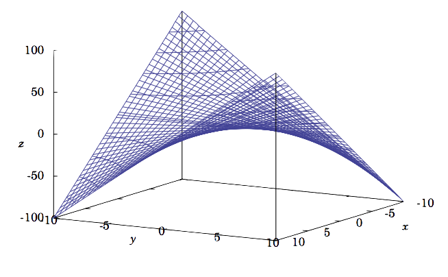
The function f(x,y)=xy has a critical point at (0,0): ∂f∂x=y=0⇒y=0, and ∂f∂y=x=0⇒x=0, so (0,0) is the only critical point. But clearly f does not have a local maximum or minimum at (0,0) since any disk around (0,0) contains points (x,y) where the values of x and y have the same sign (so that f(x,y)=xy>0=f(0,0)) and different signs (so that f(x,y)=xy<0=f(0,0)). In fact, along the path y=x in R2, f(x,y)=x2, which has a local minimum at (0,0), while along the path y=−x we have f(x,y)=−x2, which has a local maximum at (0,0). So (0,0) is an example of a saddle point, i.e. it is a local maximum in one direction and a local minimum in another direction. The graph of f(x,y) is shown in Figure 2.5.1, which is a hyperbolic paraboloid.
The following theorem gives sufficient conditions for a critical point to be a local maximum or minimum of a smooth function (i.e. a function whose partial derivatives of all orders exist and are continuous), which we will not prove here.
Theorem 2.6
Let f(x,y) be a smooth real-valued function, with a critical point at (a,b) (i.e. ∇f(a,b)=0). Define
D=∂2f∂x2(a,b)∂2f∂y2(a,b)−(∂2f∂y∂x(a,b))2
Then
- if D>0 and ∂2f∂x2(a,b)>0, then f has a local minimum at (a,b)
- if D>0 and ∂2f∂x2(a,b)<0, then f has a local maximum at (a,b)
- if D<0, then f has neither a local minimum nor a local maximum at (a,b)
- if D=0, then the test fails
If condition (c) holds, then (a,b) is a saddle point. Note that the assumption that f(x,y) is smooth means that
D=|∂2f∂x2(a,b)∂2f∂y∂x(a,b)∂2f∂x∂y(a,b)∂2f∂y2(a,b)|
since ∂2f∂y∂x=∂2f∂x∂y. Also, if D>0 then ∂2f∂x2(a,b)∂2f∂y2(a,b)=D+(∂2f∂y∂x(a,b))2>0, and so ∂2f∂x2(a,b) and ∂2f∂y2(a,b) have the same sign. This means that in parts (a) and (b) of the theorem one can replace ∂2f∂x2(a,b) by ∂2f∂y2(a,b) if desired.
Example 2.19
Find all local maxima and minima of f(x,y)=x2+xy+y2−3x.
Solution
First find the critical points, i.e. where ∇f=0. Since
∂f∂x=2x+y−3 and ∂f∂y=x+2y
then the critical points (x,y) are the common solutions of the equations
2x+y−3=0x+2y=0
which has the unique solution (x,y)=(2,−1). So (2,−1) is the only critical point.
To use Theorem 2.6, we need the second-order partial derivatives:
∂2f∂x2=2,∂2f∂y2=2,∂2f∂y∂x=1
and so
D=∂2f∂x2(2,−1)∂2f∂y2(2,−1)−(∂2f∂y∂x(2,−1))2=(2)(2)−12=3>0
and ∂2f∂x2(2,−1)=2>0. Thus, (2,−1) is a local minimum.
Example 2.20
Find all local maxima and minima of f(x,y)=xy−x3−y2.
Solution
First find the critical points, i.e. where ∇f=0. Since
∂f∂x=y−3x2 and ∂f∂y=x−2y
then the critical points (x,y) are the common solutions of the equations
y−3x2=0x−2y=0
The first equation yields y=3x2, substituting that into the second equation yields x−6x2=0, which has the solutions x=0 and x=16. So x=0⇒y=3(0)=0 and x=16⇒y=3(16)2=112. So the critical points are (x,y)=(0,0) and (x,y)=(16,112).
To use Theorem 2.6, we need the second-order partial derivatives:
∂2f∂x2=−6x,∂2f∂y2=−2,∂2f∂y∂x=1
So
D=∂2f∂x2(0,0)∂2f∂y2(0,0)−(∂2f∂y∂x(0,0))2=(−6(0))(−2)−12=−1<0
and thus (0,0) is a saddle point. Also,
D=∂2f∂x2(16,112)∂2f∂y2(16,112)−(∂2f∂y∂x(16,112))2=(−6(16))(−2)−12=1>0
and ∂2f∂x2(16,112)=−1<0. Thus, (16,112) is a local maximum.
Example 2.21
Find all local maxima and minima of f(x,y)=(x−2)4+(x−2y)2.
First find the critical points, i.e. where ∇f=0. Since
∂f∂x=4(x−2)3+2(x−2y) and ∂f∂y=−4(x−2y)
then the critical points (x,y) are the common solutions of the equations
4(x−2)3+2(x−2y)=0−4(x−2y)=0
The second equation yields x=2y, substituting that into the first equation yields 4(2y−2)3=0, which has the solution y=1, and so x=2(1)=2. Thus, (2,1) is the only critical point.
To use Theorem 2.6, we need the second-order partial derivatives:
∂2f∂x2=12(x−2)2+2,∂2f∂y2=8,∂2f∂y∂x=−4
So
D=∂2f∂x2(2,1)∂2f∂y2(2,1)−(∂2f∂y∂x(2,1))2=(2)(8)−(−4)2=0
and so the test fails. What can be done in this situation? Sometimes it is possible to examine the function to see directly the nature of a critical point. In our case, we see that f(x,y)≥0 for all (x,y), since f(x,y) is the sum of fourth and second powers of numbers and hence must be nonnegative. But we also see that f(2,1)=0. Thus f(x,y)≥0=f(2,1) for all (x,y), and hence (2,1) is in fact a global minimum for f.
Example 2.22
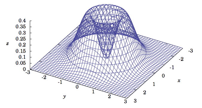
Find all local maxima and minima of f(x,y)=(x2+y2)e−(x2+y2).
Solution
First find the critical points, i.e. where ∇f=0. Since
∂f∂x=2x(1−(x2+y2))e−(x2+y2)∂f∂y=2y(1−(x2+y2))e−(x2+y2)
then the critical points are (0,0) and all points (x,y) on the unit circle x2+y2=1.
To use Theorem 2.6, we need the second-order partial derivatives:
∂2f∂x2=2[1−(x2+y2)−2x2−2x2(1−(x2+y2))]e−(x2+y2)∂2f∂y2=2[1−(x2+y2)−2y2−2y2(1−(x2+y2))]e−(x2+y2)∂2f∂y∂x=−4xy[2−(x2+y2)]e−(x2+y2)
At (0,0), we have D=4>0 and ∂2f∂x2(0,0)=2>0, so (0,0) is a local minimum. However, for points (x,y) on the unit circle x2+y2=1, we have
D=(−4x2e−1)(−4y2e−1)−(−4xye−1)2=0
and so the test fails. If we look at the graph of f(x,y), as shown in Figure 2.5.2, it looks like we might have a local maximum for (x,y) on the unit circle x2+y2=1. If we switch to using polar coordinates (r,θ) instead of (x,y) in R2, where r2=x2+y2, then we see that we can write f(x,y) as a function g(r) of the variable r alone: g(r)=r2e−r2. Then g′(r)=2r(1−r2)e−r2, so it has a critical point at r=1, and we can check that g′′(1)=−4e−1<0, so the Second Derivative Test from single-variable calculus says that r=1 is a local maximum. But r=1 corresponds to the unit circle x2+y2=1. Thus, the points (x,y) on the unit circle x2+y2=1 are local maximum points for f.