14.7: Maxima and minima
- Page ID
- 935
\( \newcommand{\vecs}[1]{\overset { \scriptstyle \rightharpoonup} {\mathbf{#1}} } \)
\( \newcommand{\vecd}[1]{\overset{-\!-\!\rightharpoonup}{\vphantom{a}\smash {#1}}} \)
\( \newcommand{\dsum}{\displaystyle\sum\limits} \)
\( \newcommand{\dint}{\displaystyle\int\limits} \)
\( \newcommand{\dlim}{\displaystyle\lim\limits} \)
\( \newcommand{\id}{\mathrm{id}}\) \( \newcommand{\Span}{\mathrm{span}}\)
( \newcommand{\kernel}{\mathrm{null}\,}\) \( \newcommand{\range}{\mathrm{range}\,}\)
\( \newcommand{\RealPart}{\mathrm{Re}}\) \( \newcommand{\ImaginaryPart}{\mathrm{Im}}\)
\( \newcommand{\Argument}{\mathrm{Arg}}\) \( \newcommand{\norm}[1]{\| #1 \|}\)
\( \newcommand{\inner}[2]{\langle #1, #2 \rangle}\)
\( \newcommand{\Span}{\mathrm{span}}\)
\( \newcommand{\id}{\mathrm{id}}\)
\( \newcommand{\Span}{\mathrm{span}}\)
\( \newcommand{\kernel}{\mathrm{null}\,}\)
\( \newcommand{\range}{\mathrm{range}\,}\)
\( \newcommand{\RealPart}{\mathrm{Re}}\)
\( \newcommand{\ImaginaryPart}{\mathrm{Im}}\)
\( \newcommand{\Argument}{\mathrm{Arg}}\)
\( \newcommand{\norm}[1]{\| #1 \|}\)
\( \newcommand{\inner}[2]{\langle #1, #2 \rangle}\)
\( \newcommand{\Span}{\mathrm{span}}\) \( \newcommand{\AA}{\unicode[.8,0]{x212B}}\)
\( \newcommand{\vectorA}[1]{\vec{#1}} % arrow\)
\( \newcommand{\vectorAt}[1]{\vec{\text{#1}}} % arrow\)
\( \newcommand{\vectorB}[1]{\overset { \scriptstyle \rightharpoonup} {\mathbf{#1}} } \)
\( \newcommand{\vectorC}[1]{\textbf{#1}} \)
\( \newcommand{\vectorD}[1]{\overrightarrow{#1}} \)
\( \newcommand{\vectorDt}[1]{\overrightarrow{\text{#1}}} \)
\( \newcommand{\vectE}[1]{\overset{-\!-\!\rightharpoonup}{\vphantom{a}\smash{\mathbf {#1}}}} \)
\( \newcommand{\vecs}[1]{\overset { \scriptstyle \rightharpoonup} {\mathbf{#1}} } \)
\(\newcommand{\longvect}{\overrightarrow}\)
\( \newcommand{\vecd}[1]{\overset{-\!-\!\rightharpoonup}{\vphantom{a}\smash {#1}}} \)
\(\newcommand{\avec}{\mathbf a}\) \(\newcommand{\bvec}{\mathbf b}\) \(\newcommand{\cvec}{\mathbf c}\) \(\newcommand{\dvec}{\mathbf d}\) \(\newcommand{\dtil}{\widetilde{\mathbf d}}\) \(\newcommand{\evec}{\mathbf e}\) \(\newcommand{\fvec}{\mathbf f}\) \(\newcommand{\nvec}{\mathbf n}\) \(\newcommand{\pvec}{\mathbf p}\) \(\newcommand{\qvec}{\mathbf q}\) \(\newcommand{\svec}{\mathbf s}\) \(\newcommand{\tvec}{\mathbf t}\) \(\newcommand{\uvec}{\mathbf u}\) \(\newcommand{\vvec}{\mathbf v}\) \(\newcommand{\wvec}{\mathbf w}\) \(\newcommand{\xvec}{\mathbf x}\) \(\newcommand{\yvec}{\mathbf y}\) \(\newcommand{\zvec}{\mathbf z}\) \(\newcommand{\rvec}{\mathbf r}\) \(\newcommand{\mvec}{\mathbf m}\) \(\newcommand{\zerovec}{\mathbf 0}\) \(\newcommand{\onevec}{\mathbf 1}\) \(\newcommand{\real}{\mathbb R}\) \(\newcommand{\twovec}[2]{\left[\begin{array}{r}#1 \\ #2 \end{array}\right]}\) \(\newcommand{\ctwovec}[2]{\left[\begin{array}{c}#1 \\ #2 \end{array}\right]}\) \(\newcommand{\threevec}[3]{\left[\begin{array}{r}#1 \\ #2 \\ #3 \end{array}\right]}\) \(\newcommand{\cthreevec}[3]{\left[\begin{array}{c}#1 \\ #2 \\ #3 \end{array}\right]}\) \(\newcommand{\fourvec}[4]{\left[\begin{array}{r}#1 \\ #2 \\ #3 \\ #4 \end{array}\right]}\) \(\newcommand{\cfourvec}[4]{\left[\begin{array}{c}#1 \\ #2 \\ #3 \\ #4 \end{array}\right]}\) \(\newcommand{\fivevec}[5]{\left[\begin{array}{r}#1 \\ #2 \\ #3 \\ #4 \\ #5 \\ \end{array}\right]}\) \(\newcommand{\cfivevec}[5]{\left[\begin{array}{c}#1 \\ #2 \\ #3 \\ #4 \\ #5 \\ \end{array}\right]}\) \(\newcommand{\mattwo}[4]{\left[\begin{array}{rr}#1 \amp #2 \\ #3 \amp #4 \\ \end{array}\right]}\) \(\newcommand{\laspan}[1]{\text{Span}\{#1\}}\) \(\newcommand{\bcal}{\cal B}\) \(\newcommand{\ccal}{\cal C}\) \(\newcommand{\scal}{\cal S}\) \(\newcommand{\wcal}{\cal W}\) \(\newcommand{\ecal}{\cal E}\) \(\newcommand{\coords}[2]{\left\{#1\right\}_{#2}}\) \(\newcommand{\gray}[1]{\color{gray}{#1}}\) \(\newcommand{\lgray}[1]{\color{lightgray}{#1}}\) \(\newcommand{\rank}{\operatorname{rank}}\) \(\newcommand{\row}{\text{Row}}\) \(\newcommand{\col}{\text{Col}}\) \(\renewcommand{\row}{\text{Row}}\) \(\newcommand{\nul}{\text{Nul}}\) \(\newcommand{\var}{\text{Var}}\) \(\newcommand{\corr}{\text{corr}}\) \(\newcommand{\len}[1]{\left|#1\right|}\) \(\newcommand{\bbar}{\overline{\bvec}}\) \(\newcommand{\bhat}{\widehat{\bvec}}\) \(\newcommand{\bperp}{\bvec^\perp}\) \(\newcommand{\xhat}{\widehat{\xvec}}\) \(\newcommand{\vhat}{\widehat{\vvec}}\) \(\newcommand{\uhat}{\widehat{\uvec}}\) \(\newcommand{\what}{\widehat{\wvec}}\) \(\newcommand{\Sighat}{\widehat{\Sigma}}\) \(\newcommand{\lt}{<}\) \(\newcommand{\gt}{>}\) \(\newcommand{\amp}{&}\) \(\definecolor{fillinmathshade}{gray}{0.9}\)Suppose a surface given by \(f(x,y)\) has a local maximum at \((x_0,y_0,z_0)\); geometrically, this point on the surface looks like the top of a hill. If we look at the cross-section in the plane \(y=y_0\), we will see a local maximum on the curve at \((x_0,z_0)\), and we know from single-variable calculus that \({\partial z\over\partial x}=0\) at this point.
Likewise, in the plane \(x=x_0\), \({\partial z\over\partial y}=0\). So if there is a local maximum at \((x_0,y_0,z_0)\), both partial derivatives at the point must be zero, and likewise for a local minimum. Thus, to find local maximum and minimum points, we need only consider those points at which both partial derivatives are 0. As in the single-variable case, it is possible for the derivatives to be 0 at a point that is neither a maximum or a minimum, so we need to test these points further.
You will recall that in the single variable case, we examined three methods to identify maximum and minimum points; the most useful is the second derivative test, though it does not always work. For functions of two variables there is also a second derivative test; again it is by far the most useful test, though it does not always work.
Suppose that the second partial derivatives of \(f(x,y)\) are continuous near \((x_0,y_0)\), and \(f_x(x_0,y_0)=f_y(x_0,y_0)=0\). We denote by \(D\) the discriminant:
\[D(x_0,y_0)=f_{xx}(x_0,y_0)f_{yy}(x_0,y_0)-f_{xy}(x_0,y_0)^2. \nonumber \]
If \(D>0\) and \(f_{xx}(x_0,y_0) < 0\) there is a local maximum at \((x_0,y_0)\); if \(D>0\) and \(f_{xx}(x_0,y_0)>0\) there is a local minimum at \((x_0,y_0)\); if \(D < 0\) there is neither a maximum nor a minimum at \((x_0,y_0)\); if \(D=0\), the test fails.
Verify that \(f(x,y)=x^2+y^2\) has a minimum at \((0,0)\).
Solution
First, we compute all the needed derivatives:
\[f_x=2x \qquad f_y=2y \qquad f_{xx}=2 \qquad f_{yy}=2 \qquad f_{xy}=0. \nonumber \]
The derivatives \(f_x\) and \(f_y\) are zero only at \((0,0)\). Applying the second derivative test there:
\[D(0,0)=f_{xx}(0,0)f_{yy}(0,0)-f_{xy}(0,0)^2= 2\cdot2-0=4>0, \nonumber \]
so there is a local minimum at \((0,0)\), and there are no other possibilities.
Find all local maxima and minima for \(f(x,y)=x^2-y^2\).
Solution
The derivatives:
\[f_x=2x \qquad f_y=-2y \qquad f_{xx}=2 \qquad f_{yy}=-2 \qquad f_{xy}=0. \nonumber \]
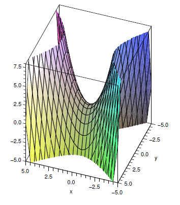
Again there is a single critical point, at \((0,0)\), and \[D(0,0)=f_{xx}(0,0)f_{yy}(0,0)-f_{xy}(0,0)^2= 2\cdot-2-0=-4 < 0, \nonumber \] so there is neither a maximum nor minimum there, and so there are no local maxima or minima. The surface is shown in Figure \(\PageIndex{1}\).

Figure \(\PageIndex{1}\): A saddle point, neither a maximum nor a minimum.
Find all local maxima and minima for \(f(x,y)=x^4+y^4\).
Solution
The derivatives:
\[f_x=4x^3 \qquad f_y=4y^3 \qquad f_{xx}=12x^2 \qquad f_{yy}=12y^2 \qquad f_{xy}=0. \nonumber \]
Again there is a single critical point, at \((0,0)\), and
\[D(0,0)=f_{xx}(0,0)f_{yy}(0,0)-f_{xy}(0,0)^2= 0\cdot0-0=0, \nonumber \]
so we get no information. However, in this case it is easy to see that there is a minimum at \((0,0)\), because \(f(0,0)=0\) and at all other points \(f(x,y)>0\).
Find all local maxima and minima for \(f(x,y)=x^3+y^3\).
Solution
The derivatives:
\[f_x=3x^2 \qquad f_y=3y^2 \qquad f_{xx}=6x^2 \qquad f_{yy}=6y^2 \qquad f_{xy}=0. \nonumber \]
Again there is a single critical point, at \((0,0)\), and
\[D(0,0)=f_{xx}(0,0)f_{yy}(0,0)-f_{xy}(0,0)^2= 0\cdot0-0=0, \nonumber \]
so we get no information. In this case, a little thought shows there is neither a maximum nor a minimum at \((0,0)\): when \(x\) and \(y\) are both positive, \(f(x,y)>0\), and when \(x\) and \(y\) are both negative, \(f(x,y) < 0\), and there are points of both kinds arbitrarily close to \((0,0)\). Alternately, if we look at the cross-section when \(y=0\), we get \(f(x,0)=x^3\), which does not have either a maximum or minimum at \(x=0\).
Suppose a box with no top is to hold a certain volume \(V\). Find the dimensions for the box that result in the minimum surface area.
Solution
The area of the box is \(A=2hw+2hl+lw\), and the volume is \(V=lwh\), so we can write the area as a function of two variables,
\[A(l,w)={2V\over l}+{2V\over w}+lw. \nonumber \]
Then
\[A_l=-{2V\over l^2}+w \quad \text{and} A_w=-{2V\over w^2}+l. \nonumber \]
If we set these equal to zero and solve, we find \(w=(2V)^{1/3}\) and \(l=(2V)^{1/3}\), and the corresponding height is \(h=V/(2V)^{2/3}\).
The second derivatives are
\[A_{ll}={4V\over l^3} \qquad A_{ww}={4V\over w^3} \qquad A_{lw}=1, \nonumber \]
so the discriminant is
\[D={4V\over l^3}{4V\over w^3}-1=4-1=3>0. \nonumber \]
Since \(A_{ll}\) is 2, there is a local minimum at the critical point. Is this a global minimum? It is, but it is difficult to see this analytically; physically and graphically it is clear that there is a minimum, in which case it must be at the single critical point.

Note that we must choose a value for \(V\) in order to graph it.
Recall that when we did single variable global maximum and minimum problems, the easiest cases were those for which the variable could be limited to a finite closed interval, for then we simply had to check all critical values and the endpoints. The previous example is difficult because there is no finite boundary to the domain of the problem---both \(w\) and \(l\) can be in \((0,\infty)\). As in the single variable case, the problem is often simpler when there is a finite boundary.
If \(f(x,y)\) is continuous on a closed and bounded subset of \(\mathbb{R}^2\), then it has both a maximum and minimum value.
As in the case of single variable functions, this means that the maximum and minimum values must occur at a critical point or on the boundary; in the two variable case, however, the boundary is a curve, not merely two endpoints.
The length of the diagonal of a box is to be 1 meter; find the maximum possible volume.
Solution
If the box is placed with one corner at the origin, and sides along the axes, the length of the diagonal is \(\sqrt{x^2+y^2+z^2}\), and the volume is
\[V=xyz=xy\sqrt{1-x^2-y^2}. \nonumber \]
Clearly, \(x^2+y^2\le 1\), so the domain we are interested in is the quarter of the unit disk in the first quadrant. Computing derivatives:
\[\eqalign{ V_x&={y-2yx^2-y^3\over\sqrt{1-x^2-y^2}}\cr V_y&={x-2xy^2-x^3\over\sqrt{1-x^2-y^2}}\cr } \nonumber \]
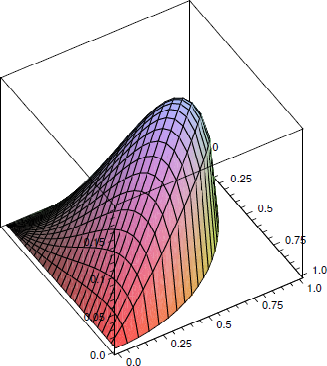
If these are both 0, then \(x=0\) or \(y=0\), or \(x=y=1/\sqrt3\). The boundary of the domain is composed of three curves: \(x=0\) for \(y\in[0,1]\); \(y=0\) for \(x\in[0,1]\); and \(x^2+y^2=1\), where \(x\ge0\) and \(y\ge0\). In all three cases, the volume \(xy\sqrt{1-x^2-y^2}\) is 0, so the maximum occurs at the only critical point \((1/\sqrt3,1/\sqrt3,1/\sqrt3)\). See Figure \(\PageIndex{2}\).

Contributors
Integrated by Justin Marshall.


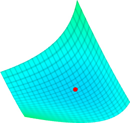
Here is the graph as rendered by Sage, as an example.