
2.3: Graph and Trees


( \newcommand{\kernel}{\mathrm{null}\,}\)
2.3.1: Undirected Graphs
In Section 1.3.4 we introduced the idea of a directed graph. Graphs consist of vertices and edges. We describe vertices and edges in much the same way as we describe points and lines in geometry: we don’t really say what vertices and edges are, but we say what they do. We just don’t have a complicated axiom system the way we do in geometry. A graph consists of a set V called a vertex set and a set E called an edge set. Each member of V is called a vertex and each member of E is called an edge. Associated with each edge are two (not necessarily different) vertices called its endpoints. We draw pictures of graphs by drawing points to represent the vertices and line segments (curved if we choose) whose endpoints are at vertices to represent the edges. In Figure 2.3.1 we show three pictures of graphs.
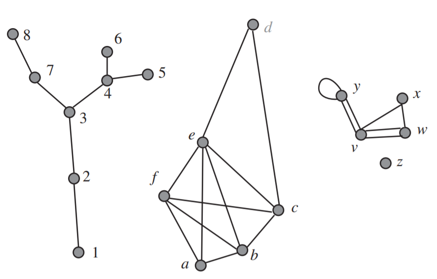
Each grey circle in the figure represents a vertex; each line segment represents an edge. You will note that we labelled the vertices; these labels are names we chose to give the vertices. We can choose names or not as we please. The third graph also shows that it is possible to have an edge that connects a vertex (like the one labelled y) to itself or it is possible to have two or more edges (like those between vertices v and y) between two vertices. The degree of a vertex is the number of times it appears as the endpoint of edges; thus the degree of y in the third graph in the figure is four.
∘ Exercise 100
In the graph on the left in Figure 2.3.1, what is the degree of each vertex?
∘ Exercise 101
For each graph in Figure 2.3.1 is the number of vertices of odd degree even or odd?
→⋅ Exercise 102
The sum of the degrees of the vertices of a (finite) graph is related in a natural way to the number of edges.
⋅ Exercise 103
What can you say about the number of vertices of odd degree in a graph? (Hint).
2.3.2: Walks and Paths in Graphs
A walk in a graph is an alternating sequence v0e1v1...eivi of vertices and edges such that edge ei connects vertices vi−1 and vi. A graph is called connected if, for any pair of vertices, there is a walk starting at one and ending at the other.
Exercise 104
Which of the graphs in Figure 2.3.1 is connected?
∘ Exercise 105
A path in a graph is a walk with no repeated vertices. Find the longest path you can in the third graph of Figure 2.3.1.
∘ Exercise 106
A cycle in a graph is a walk (with at least one edge) whose first and last vertex are equal but which has no other repeated vertices or edges. Which graphs in Figure 2.3.1 have cycles? What is the largest number of edges in a cycle in the second graph in Figure 2.3.1? What is the smallest number of edges in a cycle in the third graph in Figure 2.3.1?
∘ Exercise 107
A connected graph with no cycles is called a tree. Which graphs, if any, in Figure 2.3.1 are trees?
2.3.3: Counting Vertices, Edges, and Paths in Trees
→∙ Exercise 108
Draw some trees and on the basis of your examples, make a conjecture about the relationship between the number of vertices and edges in a tree. Prove your conjecture. (Hint).
⋅ Exercise 109
What is the minimum number of vertices of degree one in a finite tree? What is it if the number of vertices is bigger than one? Prove that you are correct. See if you can find (and give) more than one proof. (Hint).
→⋅ Exercise 110
In a tree on any number of vertices, given two vertices, how many paths can you find between them? Prove that you are correct.
→∗ Exercise 111
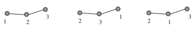
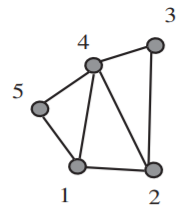
How many trees are there on the vertex set {1,2}? On the vertex set {1,2,3}? When we label the vertices of our tree, we consider the tree which has edges between vertices 1 and 2 and between vertices 2 and 3 different from the tree that has edges between vertices 1 and 3 and between 2 and 3. See Figure 2.3.2.
How many (labelled) trees are there on four vertices? How many (labelled) trees are there with five vertices? You don’t have a lot of data to guess from, but try to guess a formula for the number of labelled trees with vertex set {1,2,···,n}. (Hint).
We are now going to introduce a method to prove the formula you guessed. Given a tree with two or more vertices, labelled with positive integers, we define a sequence b1,b2,... of integers inductively as follows: If the tree has two vertices, the sequence consists of one entry, namely the label of the vertex with the larger label. Otherwise, let a1 be the lowest numbered vertex of degree 1 in the tree. Let b1 be the label of the unique vertex in the tree adjacent to a1 and write down b1. For example, in the first graph in Figure 2.3.1, a1 is 1 and b1 is 2. Given a1 through ai−1, let ai be the lowest numbered vertex of degree 1 in the tree you get by deleting a1 through ai−1 and let bi be the unique vertex in this new tree adjacent to ai. For example, in the first graph in Figure 2.3.1, a2=2 and b2=3. Then a3=5 and b3=4. We use b to stand for the sequence of bis we get in this way. In the tree (the first graph) in Figure 2.3.1, the sequence b is 2344378. (If you are unfamiliar with inductive (recursive) definition, you might want to write down some other labelled trees on eight vertices and construct the sequence of bis.)
Exercise 112
- How long will the sequence of bis be if it is computed from a tree with n vertices (labelled with 1 through n)?
- What can you say about the last member of the sequence of bis? (Hint).
- Can you tell from the sequence of bis what a1 is? (Hint).
- Find a bijection between labelled trees and something you can “count” that will tell you how many labelled trees there are on n labelled vertices. (Hint).
The sequence b1,b2,...,bn−2 in Problem 112 is called a Prüfer coding or Prüfer code for the tree. Thus the Prüfer code for the tree of Figure 2.3.1 is 234437. Notice that we do not include the term bn−1 in the Prüfer code because we know it is n. There is a good bit of interesting information encoded into the Prüfer code for a tree.
Exercise 113
What can you say about the vertices of degree one from the Prüfer code for a tree labelled with the integers from 1 to n? (Hint).
Exercise 114
What can you say about the Prüfer code for a tree with exactly two vertices of degree 1 (and perhaps some vertices with other degrees as well)? Does this characterize such trees?
→ Exercise 115
What can you determine about the degree of the vertex labelled i from the Prüfer code of the tree? (Hint).
→ Exercise 116
What is the number of (labelled) trees on n vertices with three vertices of degree 1? (Assume they are labelled with the integers 1 through n.) This problem will appear again in the next chapter after some material that will make it easier. (Hint).
2.3.4: Spanning Trees
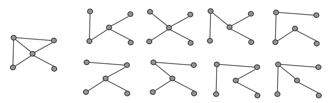
Many of the applications of trees arise from trying to find an efficient way to connect all the vertices of a graph. For example, in a telephone network, at any given time we have a certain number of wires (or microwave channels, or cellular channels) available for use. These wires or channels go from a specific place to a specific place. Thus the wires or channels may be thought of as edges of a graph and the places the wires connect may be thought of as vertices of that graph. A tree whose edges are some of the edges of a graph G and whose vertices are all of the vertices of the graph G is called a spanning tree of G. A spanning tree for a telephone network will give us a way to route calls between any two vertices in the network. In Figure 2.2.3 we show a graph and all its spanning trees.
Exercise 117
Show that every connected graph has a spanning tree. It is possible to find a proof that starts with the graph and works “down” towards the spanning tree and to find a proof that starts with just the vertices and works “up” towards the spanning tree. Can you find both kinds of proof?
2.3.5: Minimum Cost Spanning Trees
Our motivation for talking about spanning trees was the idea of finding a minimum number of edges we need to connect all the edges of a communication network together. In many cases edges of a communication network come with costs associated with them. For example, one cell-phone operator charges another one when a customer of the first uses an antenna of the other. Suppose a company has offices in a number of cities and wants to put together a communication network connecting its various locations with high-speed computer communications, but to do so at minimum cost. Then it wants to take a graph whose vertices are the cities in which it has offices and whose edges represent possible communications lines between the cities. Of course, there will not necessarily be lines between each pair of cities, and the company will not want to pay for a line connecting city i and city j if it can already connect them indirectly by using other lines it has chosen. Thus it will want to choose a spanning tree of minimum cost among all spanning trees of the communications graph. For reasons of this application, if we have a graph with numbers assigned to its edges, the sum of the numbers on the edges of a spanning tree of G will be called the cost of the spanning tree.
→ Exercise 118
Describe a method (or better, two methods different in at least one aspect) for finding a spanning tree of minimum cost in a graph whose edges are labelled with costs, the cost on an edge being the cost for including that edge in a spanning tree. Prove that your method(s) work. (Hint).
The method you used in Problem 118 is called a greedy method, because each time you made a choice of an edge, you chose the least costly edge available to you.
2.3.6: The Deletion/Contraction Recurrence for Spanning Trees
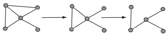
There are two operations on graphs that we can apply to get a recurrence (though a more general kind than those we have studied for sequences) which will let us compute the number of spanning trees of a graph. The operations each apply to an edge e of a graph G. The first is called deletion; we delete the edge e from the graph by removing it from the edge set. Figure 2.3.4 shows how we can delete edges from a graph to get a spanning tree.
The second operation is called contraction.
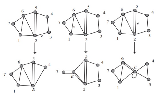
Contractions of three different edges in the same graph are shown in Figure 2.3.5. Intuitively, we contract an edge by shrinking it in length until its endpoints coincide; we let the rest of the graph “go along for the ride.” To be more precise, we contract the edge e with endpoints v and w as follows:
- remove all edges having either v or w or both as an endpoint from the edge set,
- remove v and w from the vertex set,
- add a new vertex E to the vertex set,
- add an edge from E to each remaining vertex that used to be an endpoint of an edge whose other endpoint was v or w, and add an edge from E to E for any edge other than e whose endpoints were in the set {v,w}.
We use G−e (read as G minus e) to stand for the result of deleting e from G, and we use G/e (read as G contract e) to stand for the result of contracting e from G.
→⋅ Exercise 119
- How do the number of spanning trees of G not containing the edge e and the number of spanning trees of G containing e relate to the number of spanning trees of G−e and G/e? (Hint).
- Use #(G) to stand for the number of spanning trees of G (so that, for example, #(G/e) stands for the number of spanning trees of G/e). Find an expression for #(G) in terms of #(G/e) and #(G−e). This expression is called the deletion-contraction recurrence.
- Use the recurrence of the previous part to compute the number of spanning trees of the graph in Figure 2.3.6
2.3.7: Shortest Paths in Graphs
Suppose that a company has a main office in one city and regional offices in other cities. Most of the communication in the company is between the main office and the regional offices, so the company wants to find a spanning tree that minimizes not the total cost of all the edges, but rather the cost of communication between the main office and each of the regional offices. It is not clear that such a spanning tree even exists. This problem is a special case of the following. We have a connected graph with nonnegative numbers assigned to its edges. (In this situation these numbers are often called weights.) The (weighted) length of a path in the graph is the sum of the weights of its edges. The distance between two vertices is the least (weighted) length of any path between the two vertices. Given a vertex v, we would like to know the distance between v and each other vertex, and we would like to know if there is a spanning tree in G such that the length of the path in the spanning tree from v to each vertex x is the distance from v to x in G.
Exercise 120
Show that the following algorithm (known as Dijkstra’s algorithm) applied to a weighted graph whose vertices are labelled 1 to n gives, for each i, the distance from vertex 1 to i as d(i).
- Let d(1)=0. Let d(i)=1 for all other i. Let v(1)=1. Let v(j)=0 for all other j. For each i and j, let w(i,j) be the minimum weight of an edge between i and j, or 1 if there are no such edges. Let k=1. Let t=1.
- For each i, if d(i)>d(k)+w(k,i) let d(i)=d(k)+w(k,i).
- Among those i with v(i)=0, choose one with d(i) a minimum, and let k=i. Increase t by 1. Let v(i)=1.
- Repeat the previous two steps until t=n.
Exercise 121
Is there a spanning tree such that the distance from vertex 1 to vertex i given by the algorithm in Problem 120 is the distance from vertex 1 to vertex i in the tree (using the same weights on the edges, of course)?