11.5: Graphs of Polar Equations

In this section, we discuss how to graph equations in polar coordinates on the rectangular coordinate plane. Since any given point in the plane has infinitely many different representations in polar coordinates, our ‘Fundamental Graphing Principle’ in this section is not as clean as it was for graphs of rectangular equations on page 23. We state it below for completeness.

The Fundamental Graphing Principle for Polar Equations

The graph of an equation in polar coordinates is the set of points which satisfy the equation. That is, a point \(P(r, \theta)\) is on the graph of an equation if and only if there is a representation of \(P\), say \(\left(r^{\prime}, \theta^{\prime}\right)\), such that \(r^{\prime}\) and \(\theta^{\prime}\) satisfy the equation.

Our first example focuses on some of the more structurally simple polar equations.

Example 11.5.1

Graph the following polar equations.

1. \(r = 4\)
2. \(r=-3 \sqrt{2}\)
3. \(\theta=\frac{5 \pi}{4}\)
4. \(\theta=-\frac{3 \pi}{2}\)

Solution

In each of these equations, only one of the variables \(r\) and \(\theta\) is present making the other variable free.¹ This makes these graphs easier to visualize than others.

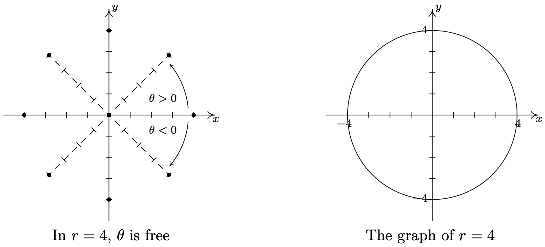
1. In the equation \(r = 4\), \(\theta\) is free. The graph of this equation is, therefore, all points which have a polar coordinate representation \((4, \theta)\), for any choice of \(\theta\). Graphically this translates into tracing out all of the points 4 units away from the origin. This is exactly the definition of circle, centered at the origin, with a radius of 4.

   

2. Once again we have \(\theta\) being free in the equation \(r=-3 \sqrt{2}\). Plotting all of the points of the form \((-3 \sqrt{2}, \theta)\) gives us a circle of radius \(3 \sqrt{2}\) centered at the origin.

   

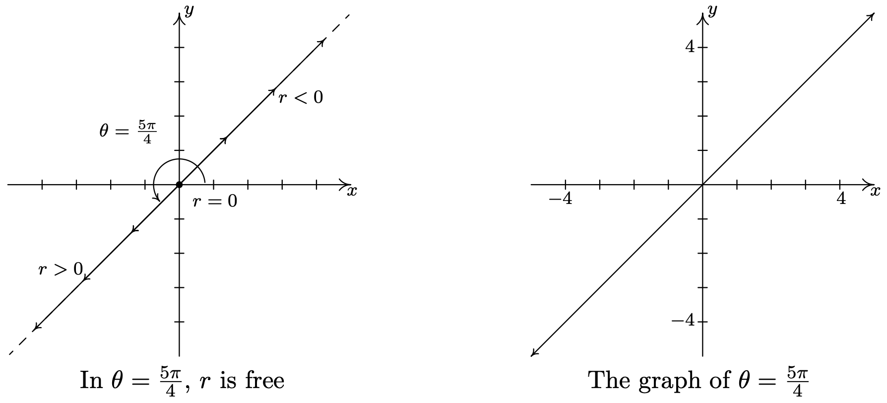
3. In the equation \(\theta=\frac{5 \pi}{4}\), \(r\) is free, so we plot all of the points with polar representation \(\left(r, \frac{5 \pi}{4}\right)\). What we find is that we are tracing out the line which contains the terminal side of \(\theta=\frac{5 \pi}{4}\) when plotted in standard position.

   

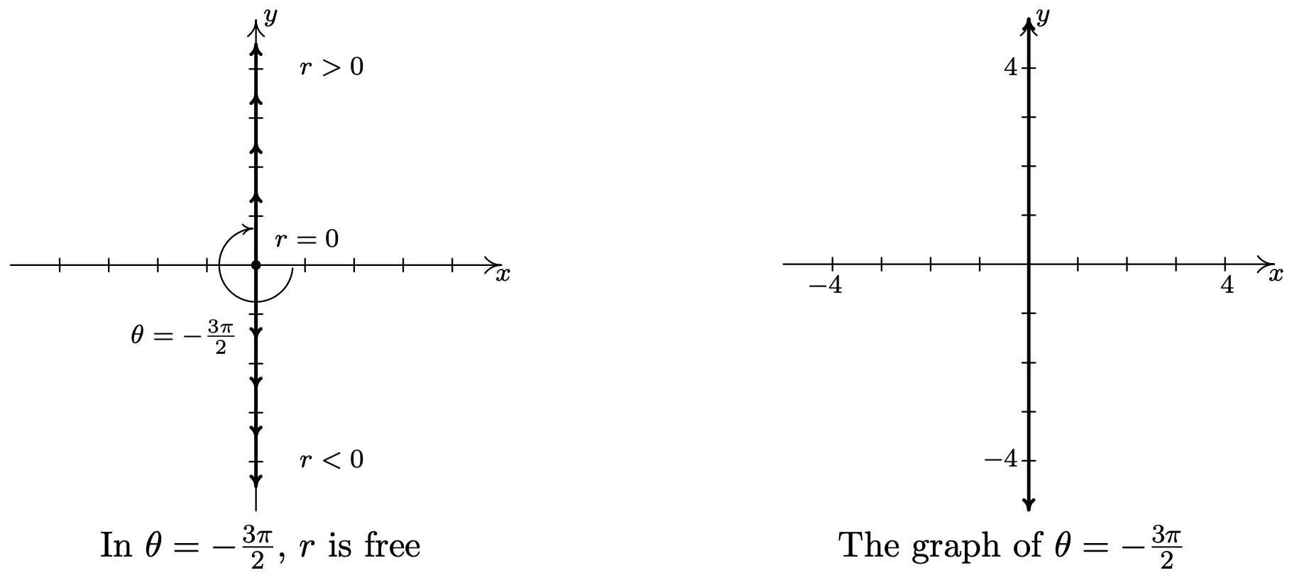
4. As in the previous example, the variable \(r\) is free in the equation \(\theta=-\frac{3 \pi}{2}\). Plotting \(\left(r,-\frac{3 \pi}{2}\right)\) for various values of \(r\) shows us that we are tracing out the \(y\)-axis.

   

Hopefully, our experience in Example 11.5.1 makes the following result clear.

Theorem 11.8. Graphs of Constant \(r\) and \(\theta\)

Suppose \(a\) and \(\alpha\) are constants, \(a \neq 0\).

• The graph of the polar equation \(r = a\) on the Cartesian plane is a circle centered at the origin of radius \(|a|\).
• The graph of the polar equation \(\theta=\alpha\) on the Cartesian plane is the line containing the terminal side of \(\alpha\) when plotted in standard position.

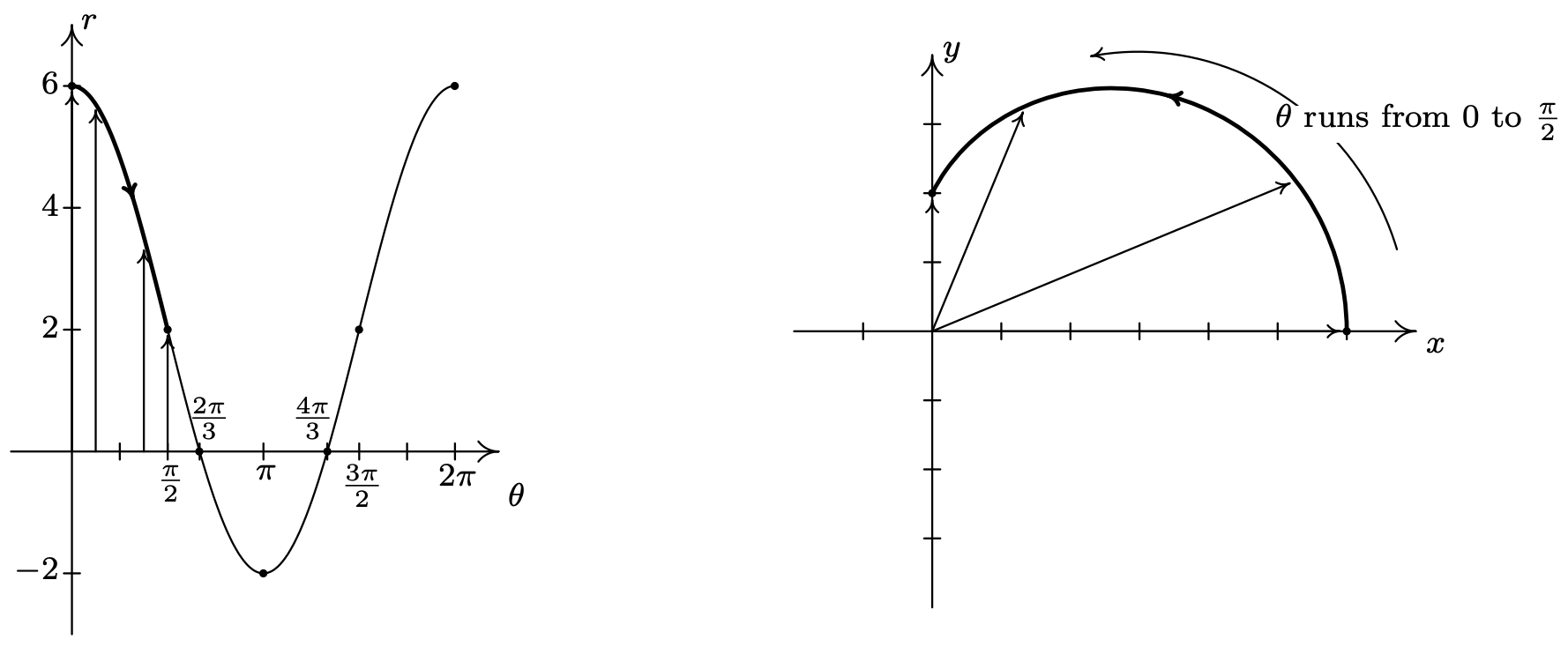
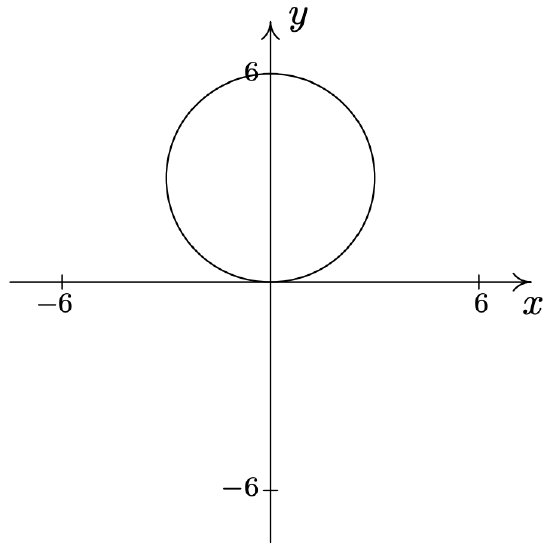
Suppose we wish to graph \(r=6 \cos (\theta)\). A reasonable way to start is to treat \(\theta\) as the independent variable, \(r\) as the dependent variable, evaluate \(r=f(\theta)\) at some ‘friendly’ values of \(\theta\) and plot the resulting points.² We generate the table below.

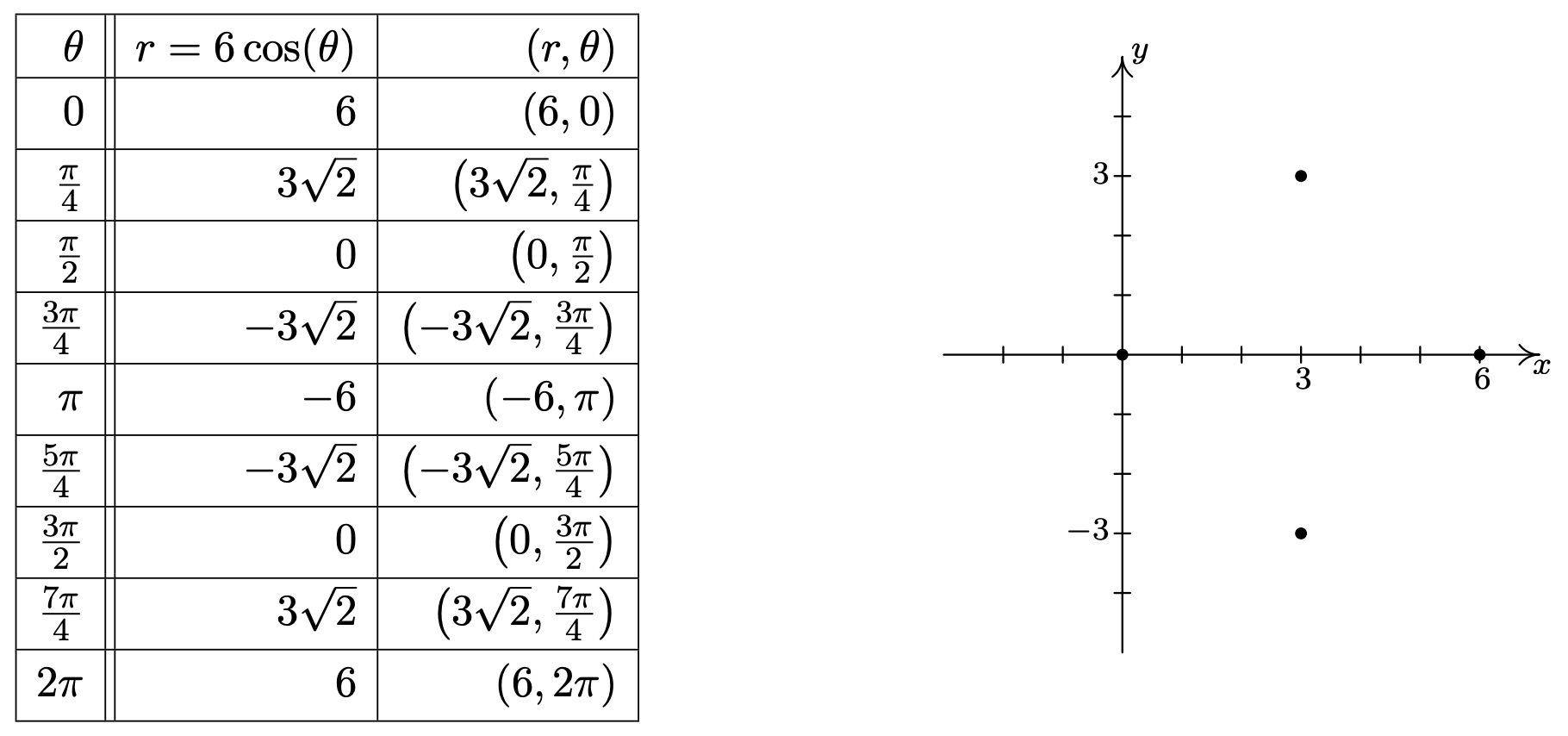
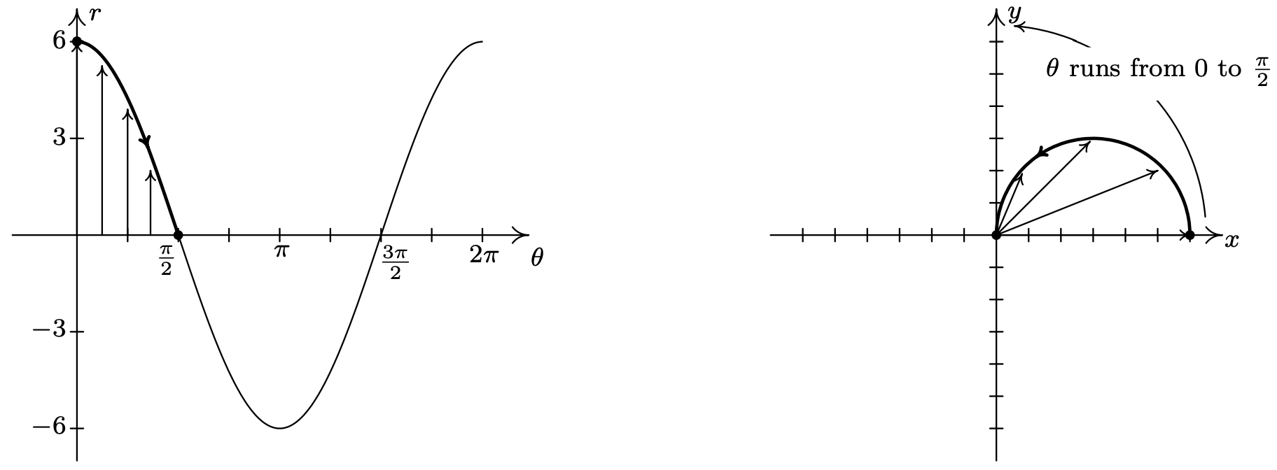
Despite having nine ordered pairs, we get only four distinct points on the graph. For this reason, we employ a slightly different strategy. We graph one cycle of \(r=6 \cos (\theta)\) on the \(\theta r-\mathrm{plane}\)³ and use it to help graph the equation on the \(xy\)-plane. We see that as \(\theta\) ranges from 0 to \(\frac{\pi}{2}\), \(r\) ranges from 6 to 0. In the \(xy\)-plane, this means that the curve starts 6 units from the origin on the positive \(x\)-axis \((\theta=0)\) and gradually returns to the origin by the time the curve reaches the \(y\)-axis \(\left(\theta=\frac{\pi}{2}\right)\). The arrows drawn in the figure below are meant to help you visualize this process. In the \(\theta r \text {-plane }\), the arrows are drawn from the \(\theta \text {-axis }\) to the curve \(r=6 \cos (\theta)\). In the \(xy\)-plane, each of these arrows starts at the origin and is rotated through the corresponding angle \(\theta\), in accordance with how we plot polar coordinates. It is a less-precise way to generate the graph than computing the actual function values, but it is markedly faster.

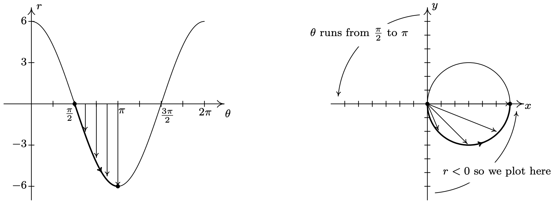
Next, we repeat the process as \(\theta\) ranges from \(\frac{\pi}{2}\) to \(\pi\). Here, the \(r\) values are all negative. This means that in the \(xy\)-plane, instead of graphing in Quadrant II, we graph in Quadrant IV, with all of the angle rotations starting from the negative \(x\)-axis.

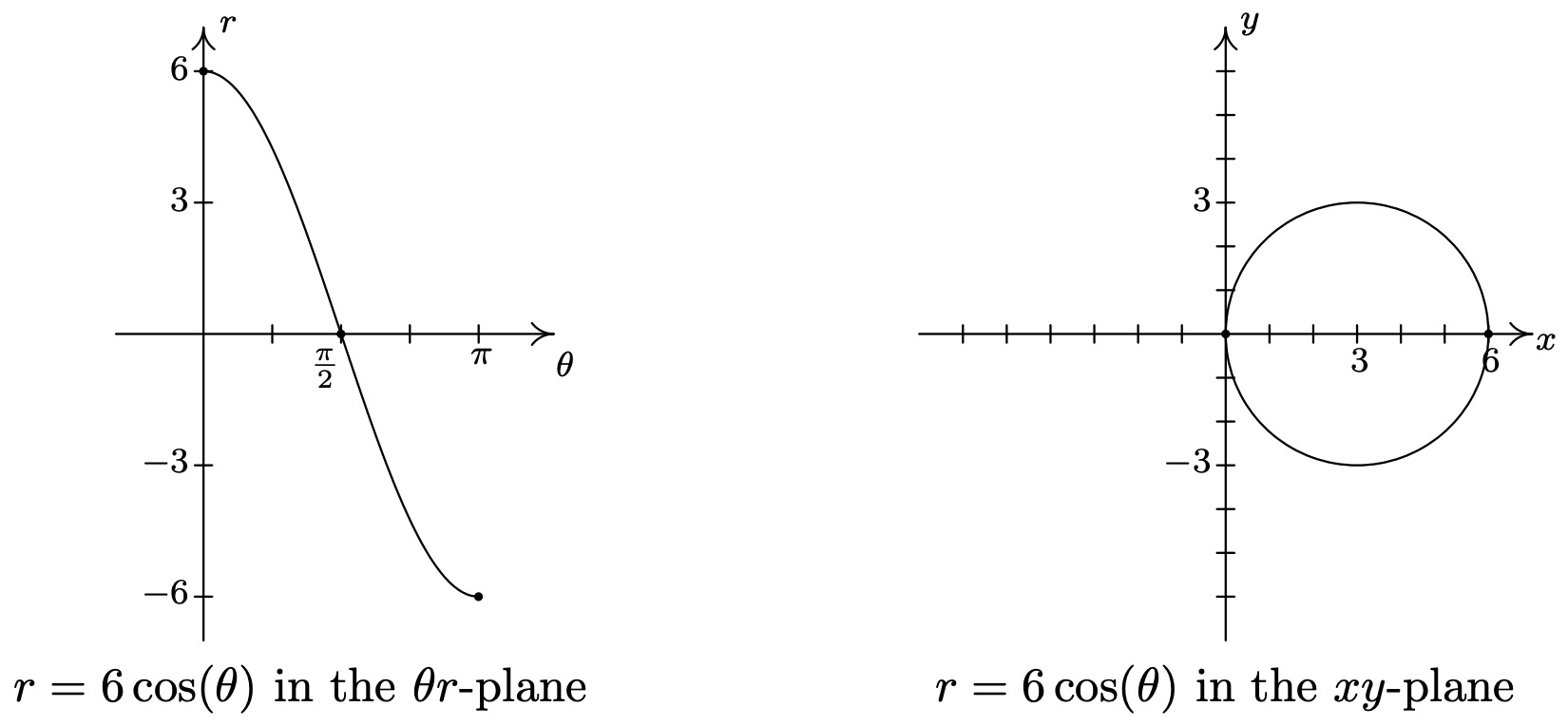
As \(\theta\) ranges from \(\pi\) to \(\frac{3 \pi}{2}\), the \(r\) values are still negative, which means the graph is traced out in Quadrant I instead of Quadrant III. Since the \(|r|\) for these values of \(\theta\) match the \(r\) values for \(\theta\) in \(\left[0, \frac{\pi}{2}\right]\), we have that the curve begins to retrace itself at this point. Proceeding further, we find that when \(\frac{3 \pi}{2} \leq \theta \leq 2 \pi\), we retrace the portion of the curve in Quadrant IV that we first traced out as \(\frac{\pi}{2} \leq \theta \leq \pi\). The reader is invited to verify that plotting any range of \(\theta\) outside the interval \([0, \pi]\) results in retracting some portion of the curve.⁴ We present the final graph below.

Example 11.5.2

Graph the following polar equations.

1. \(r=4-2 \sin (\theta)\)
2. \(r=2+4 \cos (\theta)\)
3. \(r=5 \sin (2 \theta)\)
4. \(r^{2}=16 \cos (2 \theta)\)

Solution

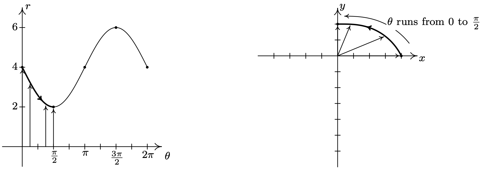
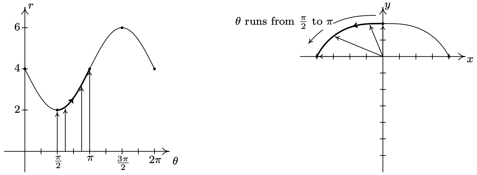
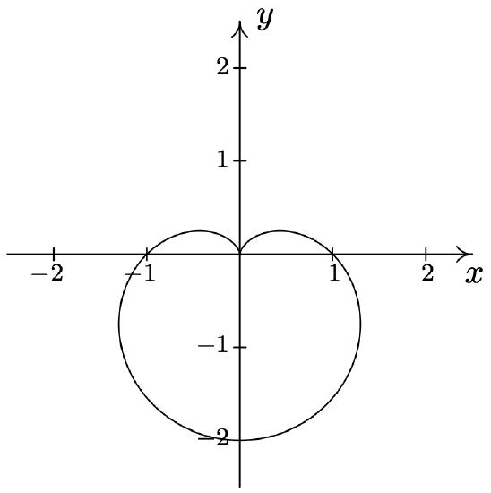
1. We first plot the fundamental cycle of \(r=4-2 \sin (\theta)\) on the \(\theta r \text {-axes }\). To help us visualize what is going on graphically, we divide up \([0,2 \pi]\) into the usual four subintervals \(\left[0, \frac{\pi}{2}\right],\left[\frac{\pi}{2}, \pi\right]\), \(\left[\pi, \frac{3 \pi}{2}\right]\) and \(\left[\frac{3 \pi}{2}, 2 \pi\right]\), and proceed as we did above. As \(\theta\) ranges from 0 to \(\frac{\pi}{2}\), \(r\) decreases from 4 to 2. This means that the curve in the \(xy\)-plane starts 4 units from the origin on the positive \(x\)-axis and gradually pulls in towards the origin as it moves towards the positive \(y\)-axis.

   

   Next, as \(\theta\) runs from \(\frac{\pi}{2}\) to \(\pi\), we see that \(r\) increases from 2 to 4. Picking up where we left off, we gradually pull the graph away from the origin until we reach the negative \(x\)-axis.

   

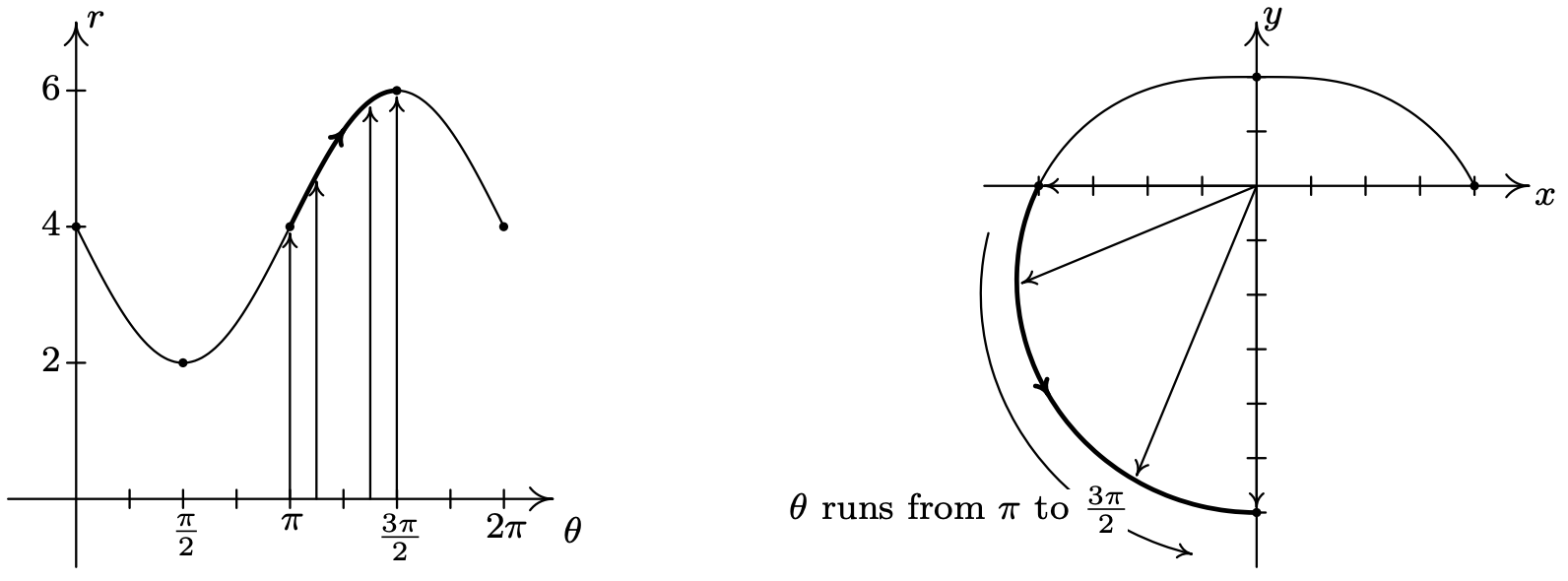
   Over the interval \(\left[\pi, \frac{3 \pi}{2}\right]\), we see that \(r\) increases from 4 to 6. On the \(xy\)-plane, the curve sweeps out away from the origin as it travels from the negative \(x\)-axis to the negative \(y\)-axis.

   

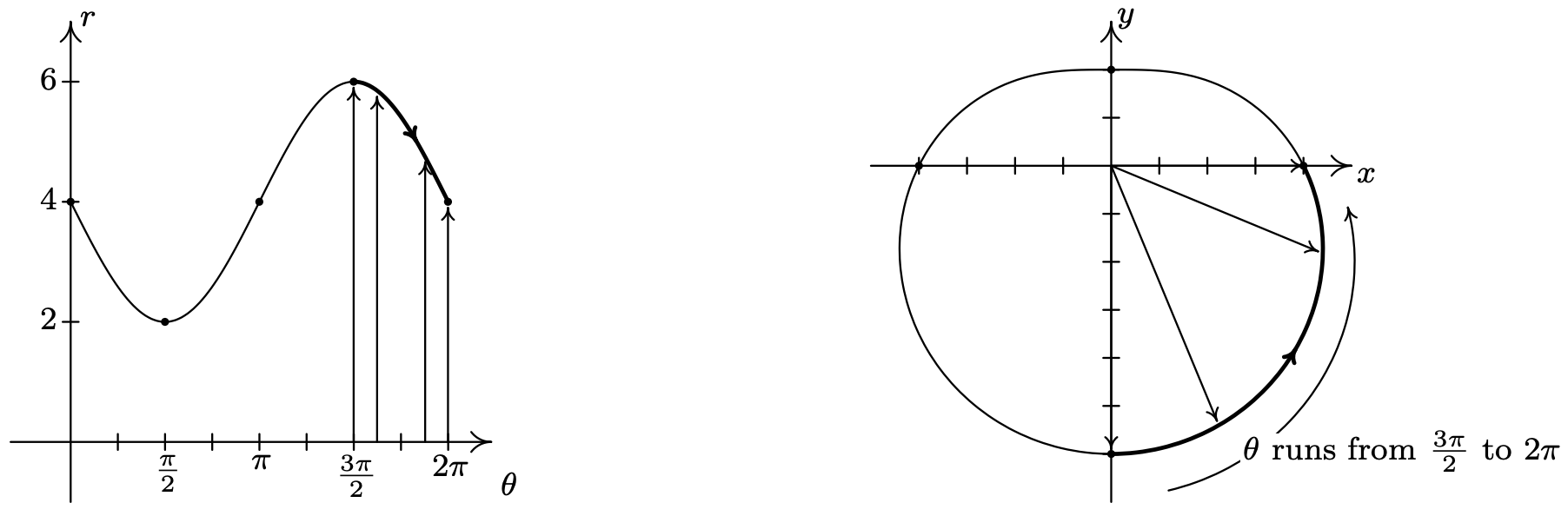
   Finally, as \(\theta\) takes on values from \(\frac{3 \pi}{2}\) to \(2 \pi\), \(r\) decreases from 6 back to 4. The graph on the \(xy\)-plane pulls in from the negative \(y\)-axis to finish where we started.

   

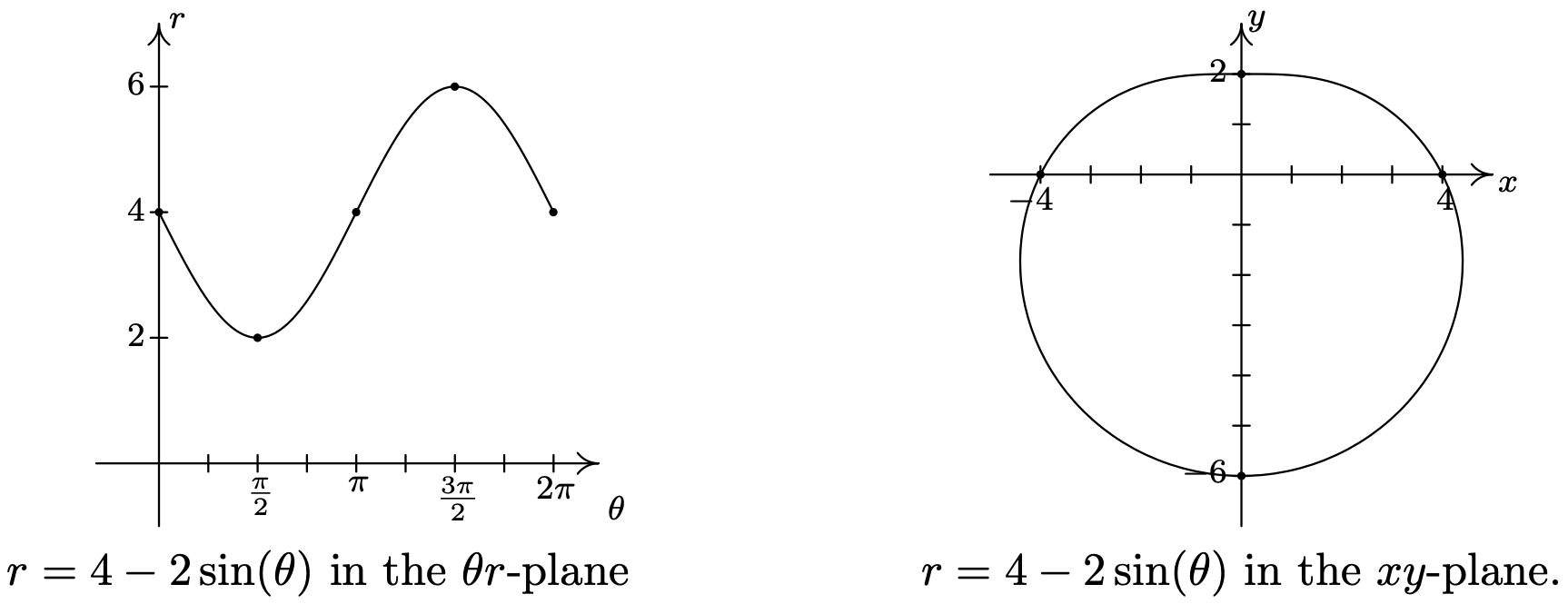
   We leave it to the reader to verify that plotting points corresponding to values of \(\theta\) outside the interval \([0,2 \pi]\) results in retracing portions of the curve, so we are finished.

   

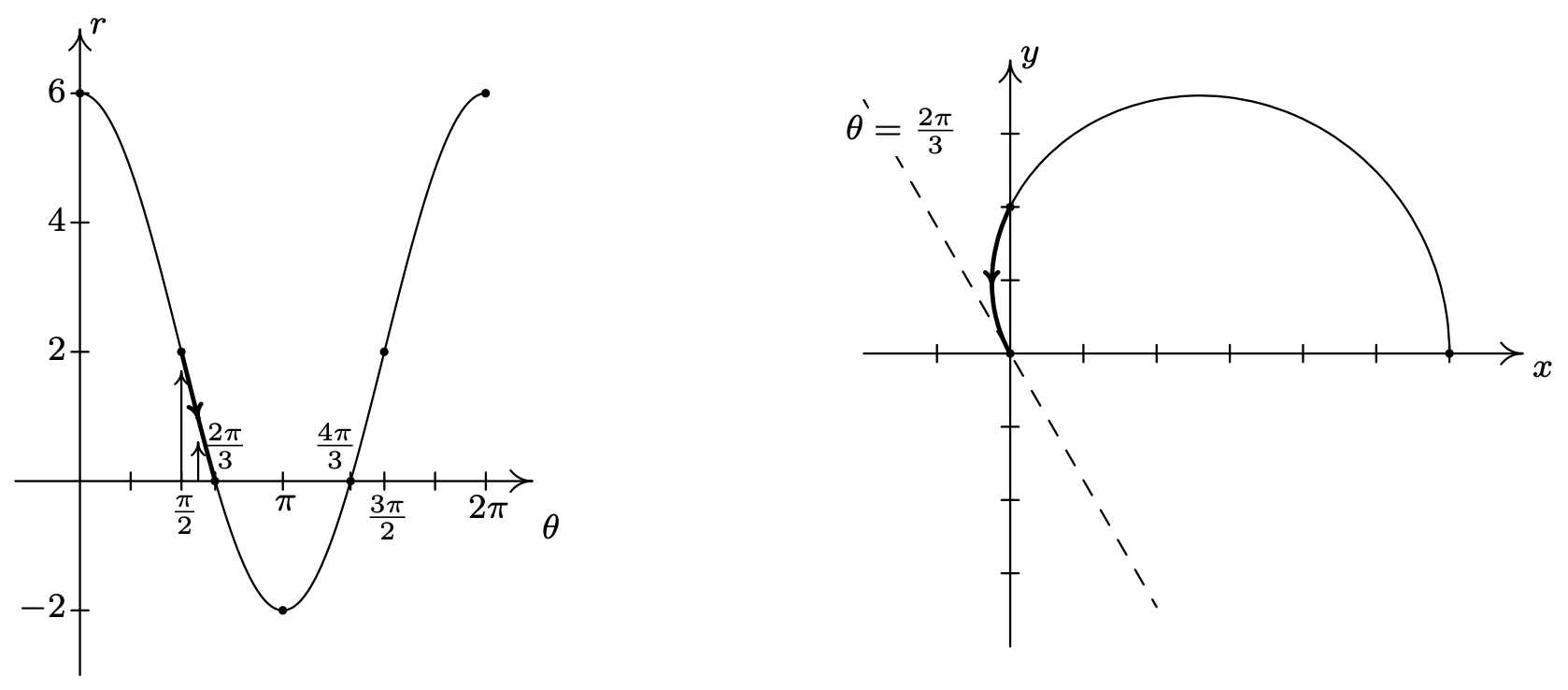
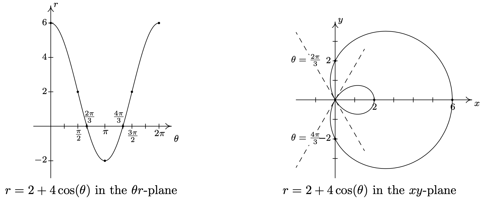
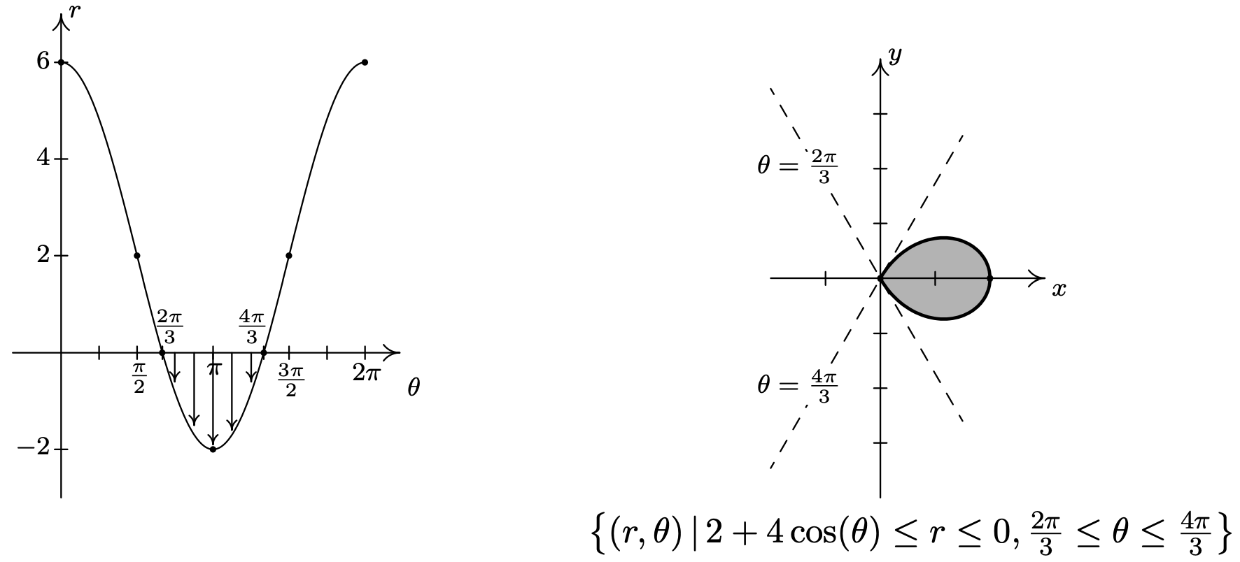
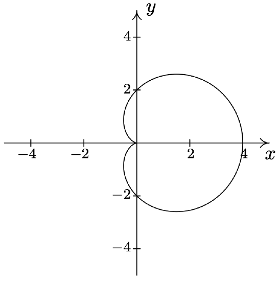
2. The first thing to note when graphing \(r=2+4 \cos (\theta)\) on the \(\theta r \text {-plane }\) over the interval \([0,2 \pi]\) is that the graph crosses through the \(\theta \text {-axis }\). This corresponds to the graph of the curve passing through the origin in the \(x y \text {-plane }\), and our first task is to determine when this happens. Setting \(r = 0\) we get \(2+4 \cos (\theta)=0\), or \(\cos (\theta)=-\frac{1}{2}\). Solving for \(\theta\) in \([0,2 \pi]\) gives \(\theta=\frac{2 \pi}{3}\) and \(\theta=\frac{4 \pi}{3}\). Since these values of \(\theta\) are important geometrically, we break the interval \([0,2 \pi]\) into six subintervals: \(\left[0, \frac{\pi}{2}\right],\left[\frac{\pi}{2}, \frac{2 \pi}{3}\right],\left[\frac{2 \pi}{3}, \pi\right],\left[\pi, \frac{4 \pi}{3}\right],\left[\frac{4 \pi}{3}, \frac{3 \pi}{2}\right] \text { and }\left[\frac{3 \pi}{2}, 2 \pi\right]\). As \(\theta\) ranges from 0 to \(\frac{\pi}{2}\), \(r\) decreases from 6 to 2. Plotting this on the \(xy\)-plane, we start 6 units out from the origin on the positive \(x\)-axis and slowly pull in towards the positive \(y\)-axis.

   

   On the interval \(\left[\frac{\pi}{2}, \frac{2 \pi}{3}\right]\), \(r\) decreases from 2 to 0, which means the graph is heading into (and will eventually cross through) the origin. Not only do we reach the origin when \(\theta=\frac{2 \pi}{3}\), a theorem from Calculus⁵ states that the curve hugs the line \(\theta=\frac{2 \pi}{3}\) as it approaches the origin.

   

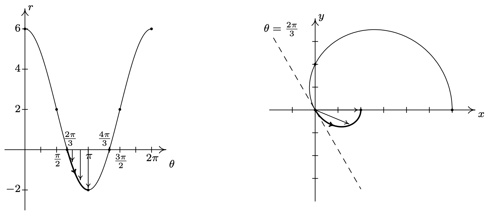
   On the interval \(\left[\frac{2 \pi}{3}, \pi\right]\), \(r\) ranges from 0 to −2. Since \(r \leq 0\), the curve passes through the origin in the \(xy\)-plane, following the line \(\theta=\frac{2 \pi}{3}\) and continues upwards through Quadrant IV towards the positive \(x\)-axis.⁶ Since \(|r|\) is increasing from 0 to 2, the curve pulls away from the origin to finish at a point on the positive \(x\)-axis.

   

   Next, as \(\theta\) progresses from \(\pi\) to \(\frac{4 \pi}{3}\), \(r\) ranges from −2 to 0. Since \(r \leq 0\), we continue our graph in the first quadrant, heading into the origin along the line \(\theta=\frac{4 \pi}{3}\).

   

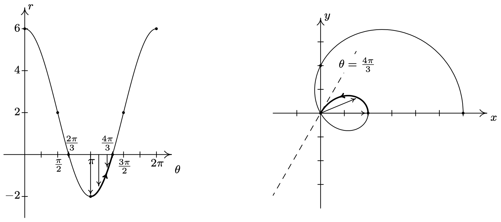
   On the interval \(\left[\frac{4 \pi}{3}, \frac{3 \pi}{2}\right]\), \(r\) returns to positive values and increases from 0 to 2. We hug the line \(\theta=\frac{4 \pi}{3}\) as we move through the origin and head towards the negative \(y\)-axis.

   

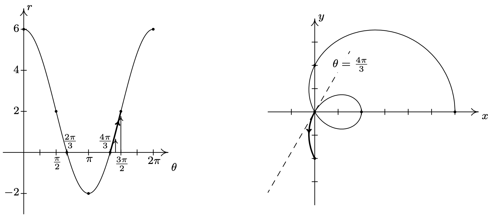
   As we round out the interval, we find that as \(\theta\) runs through \(\frac{3 \pi}{2}\) to \(2 \pi\), \(r\) increases from 2 out to 6, and we end up back where we started, 6 units from the origin on the positive \(x\)-axis.

   

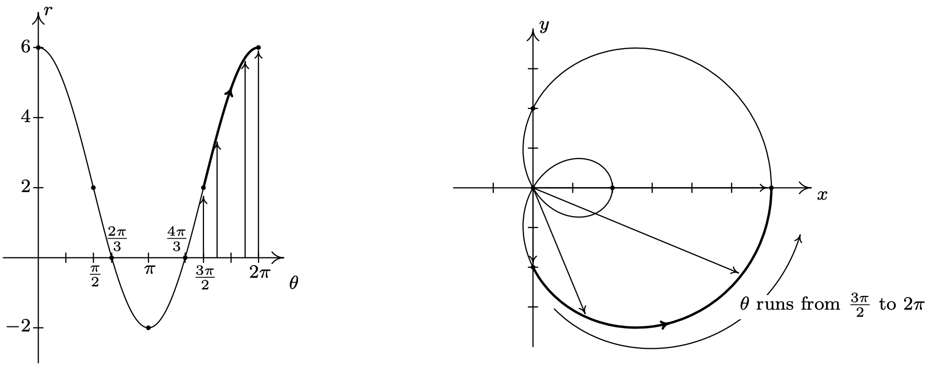
   Again, we invite the reader to show that plotting the curve for values of \(\theta\) outside \([0,2 \pi]\) results in retracing a portion of the curve already traced. Our final graph is below.

   

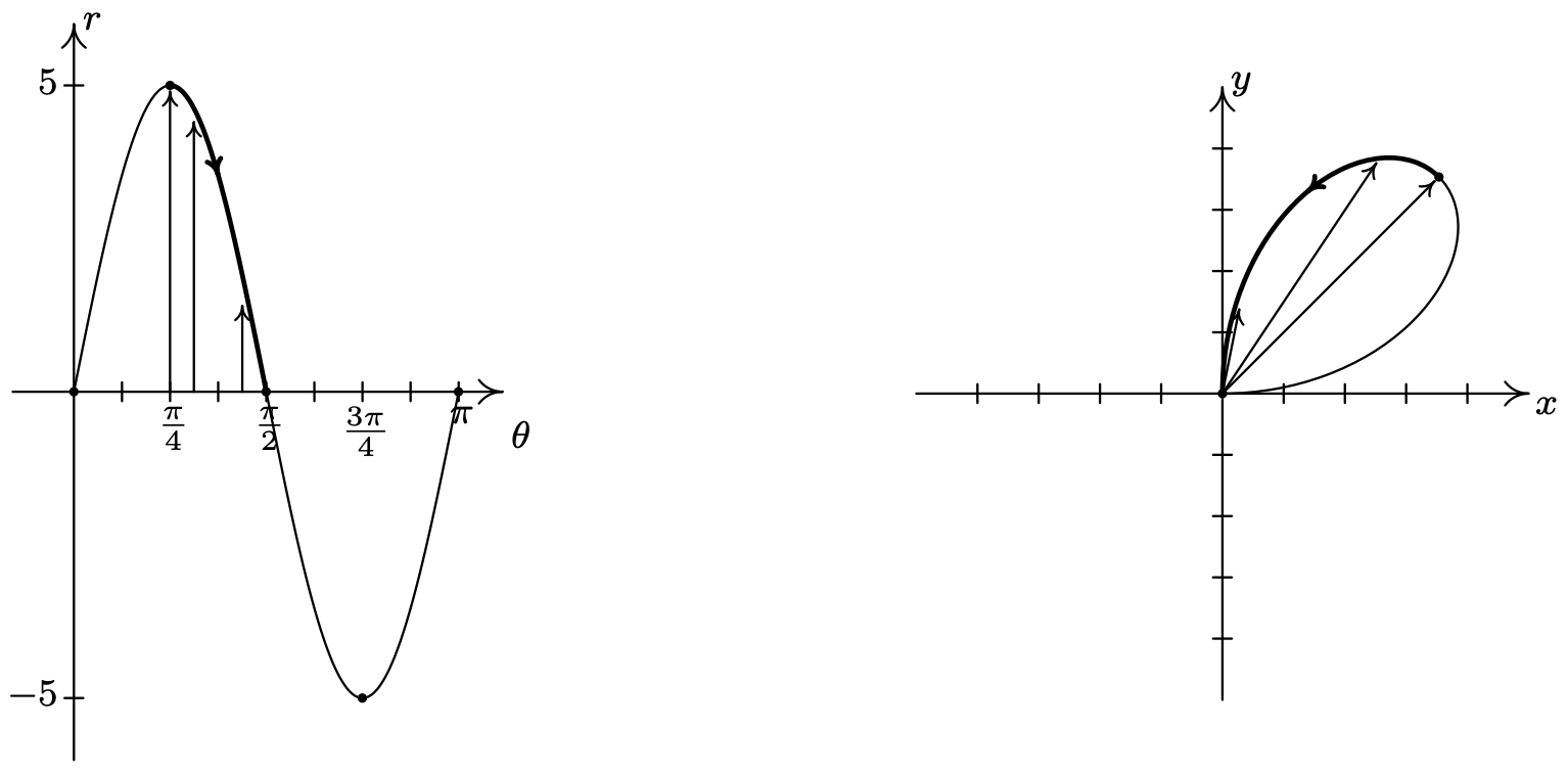
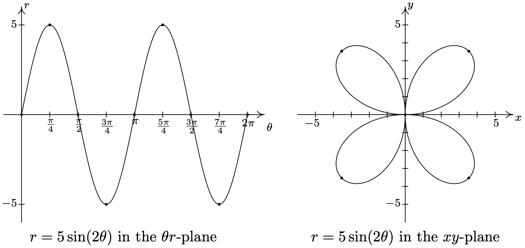
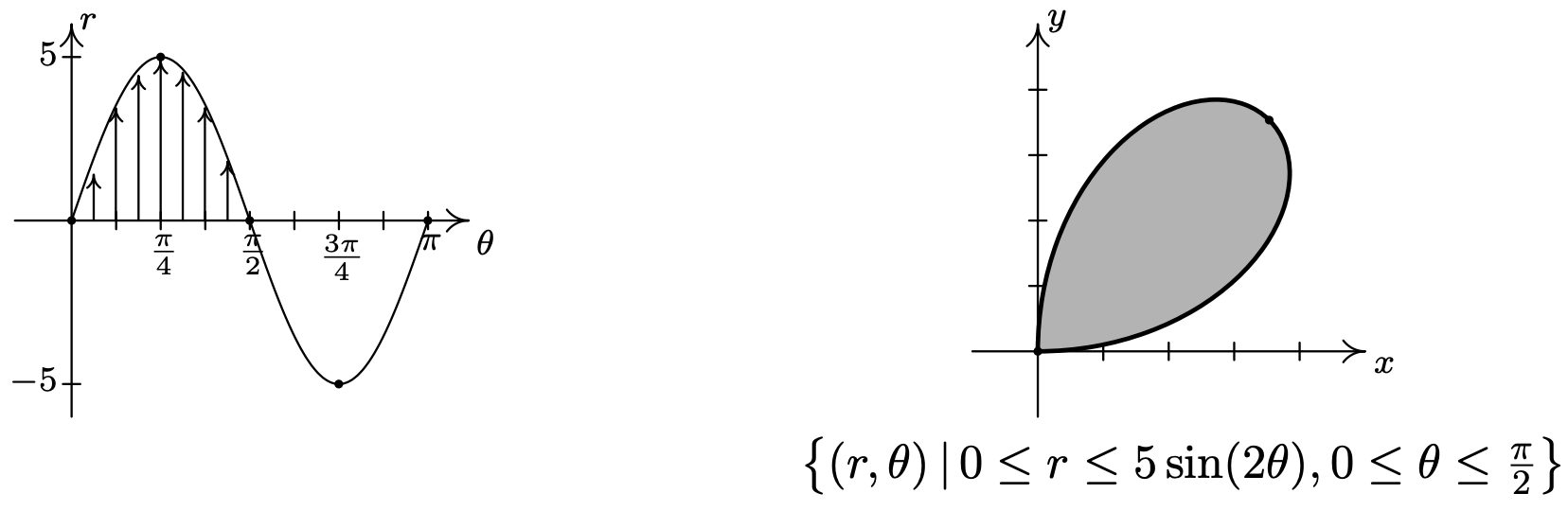
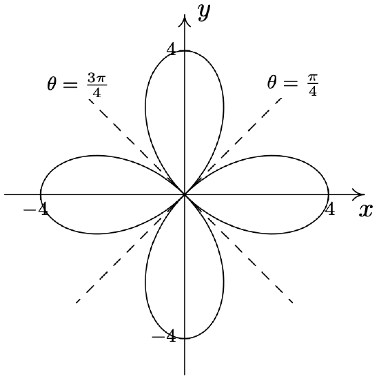
3. As usual, we start by graphing a fundamental cycle of \(r=5 \sin (2 \theta)\) in the \(\theta r \text {-plane }\), which in this case, occurs as \(\theta\) ranges from 0 to \(\pi\). We partition our interval into subintervals to help us with the graphing, namely \(\left[0, \frac{\pi}{4}\right],\left[\frac{\pi}{4}, \frac{\pi}{2}\right],\left[\frac{\pi}{2}, \frac{3 \pi}{4}\right] \text { and }\left[\frac{3 \pi}{4}, \pi\right]\). As \(\theta\) ranges from 0 to \(\frac{\pi}{4}\), \(r\) increases from 0 to 5. This means that the graph of \(r=5 \sin (2 \theta)\) in the \(xy\)-plane starts at the origin and gradually sweeps out so it is 5 units away from the origin on the line \(\theta=\frac{\pi}{4}\).

   

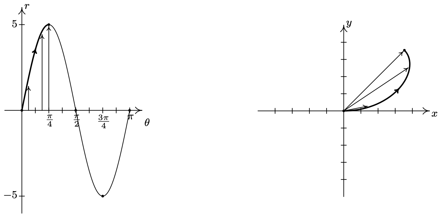
   Next, we see that \(r\) decreases from 5 to 0 as \(\theta\) runs through \(\left[\frac{\pi}{4}, \frac{\pi}{2}\right]\), and furthermore, \(r\) is heading negative as \(\theta\) crosses \(\frac{\pi}{2}\). Hence, we draw the curve hugging the line \(\theta=\frac{\pi}{2}\) (the \(y\)-axis) as the curve heads to the origin.

   

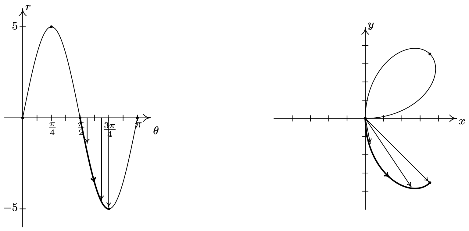
   As \(\theta\) runs from \(\frac{\pi}{2}\) to \(\frac{3 \pi}{4}\) \(r\) becomes negative and ranges from 0 to −5. Since \(r \leq 0\), the curve pulls away from the negative \(y\)-axis into Quadrant IV.

   

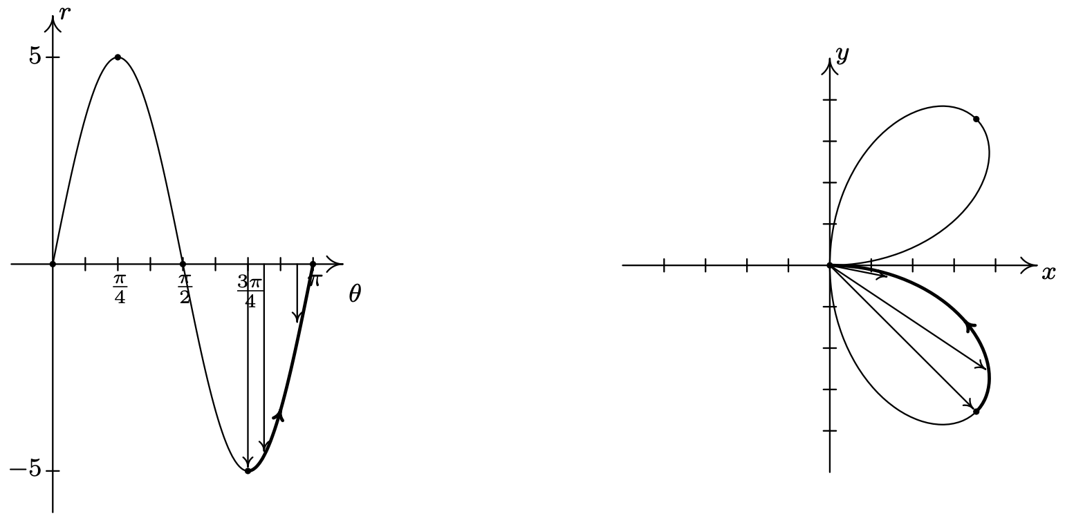
   For \(\frac{3 \pi}{4} \leq \theta \leq \pi\), \(r\) increases from −5 to 0, so the curve pulls back to the origin.

   

   Even though we have finished with one complete cycle of \(r=5 \sin (2 \theta)\), if we continue plotting beyond \(\theta=\pi\), we find that the curve continues into the third quadrant! Below we present a graph of a second cycle of \(r=5 \sin (2 \theta)\) which continues on from the first. The boxed labels on the \(\theta \text {-axis }\) correspond to the portions with matching labels on the curve in the \(x y \text {-plane }\).

   

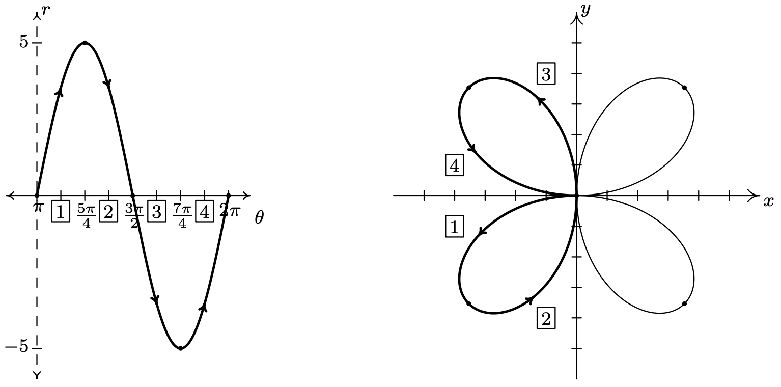
   We have the final graph below.

   

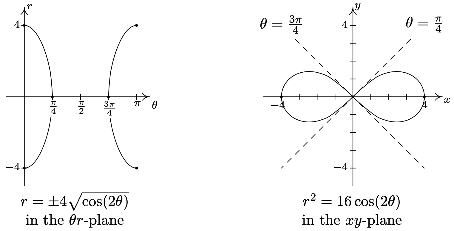
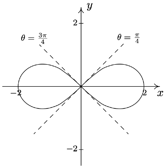
4. Graphing \(r^{2}=16 \cos (2 \theta)\) is complicated by the \(r^{2}\), so we solve to get \(r=\pm \sqrt{16 \cos (2 \theta)}=\pm4\sqrt{\cos(2\theta)}\). How do we sketch such a curve? First off, we sketch a fundamental period of \(r=\cos (2 \theta)\) which we have dotted in the figure below. When \(\cos (2 \theta)<0\), \(\sqrt{\cos (2 \theta)}\) is undefined, so we don’t have any values on the interval \(\left(\frac{\pi}{4}, \frac{3 \pi}{4}\right)\). On the intervals which remain, \(\cos (2 \theta)\) ranges from 0 to 1, inclusive. Hence \(\sqrt{\cos (2 \theta)}\) ranges from 0 to 1 as well.⁷ From this, we know \(r=\pm 4 \sqrt{\cos (2 \theta)}\) ranges continuously from 0 to \(\pm 4\), respectively. Below we graph both \(r=4 \sqrt{\cos (2 \theta)}\) and \(r=-4 \sqrt{\cos (2 \theta)}\) on the \(\theta r\) plane and use them to sketch the corresponding pieces of the curve \(r^{2}=16 \cos (2 \theta)\) in the \(xy\)-plane. As we have seen in earlier examples, the lines \(\theta=\frac{\pi}{4}\) and \(\theta=\frac{3 \pi}{4}\), which are the zeros of the functions \(r=\pm 4 \sqrt{\cos (2 \theta)}\), serve as guides for us to draw the curve as is passes through the origin.

   

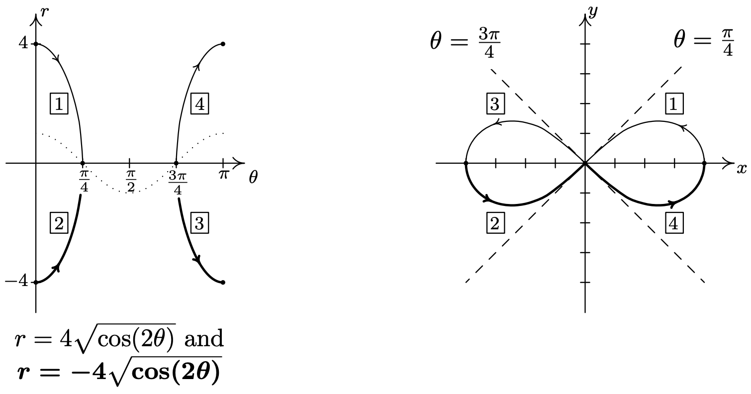
   As we plot points corresponding to values of \(\theta\) outside of the interval \([0, \pi]\), we find ourselves retracing parts of the curve,⁸ so our final answer is below.

   

A few remarks are in order. First, there is no relation, in general, between the period of the function \(f(\theta)\) and the length of the interval required to sketch the complete graph of \(r=f(\theta)\) in the \(xy\)-plane. As we saw on page 941, despite the fact that the period of \(f(\theta)=6 \cos (\theta)\) is \(2 \pi\), we sketched the complete graph of \(r=6 \cos (\theta)\) in the \(xy\)-plane just using the values of \(\theta\) as \(\theta\) ranged from 0 to \(\pi\). In Example 11.5.2, number 3, the period of \(f(\theta)=5 \sin (2 \theta)\) is \(\pi\), but in order to obtain the complete graph of \(r=5 \sin (2 \theta)\), we needed to run \(\theta\) from 0 to \(2 \pi\). While many of the ‘common’ polar graphs can be grouped into families,⁹ the authors truly feel that taking the time to work through each graph in the manner presented here is the best way to not only understand the polar coordinate system, but also prepare you for what is needed in Calculus. Second, the symmetry seen in the examples is also a common occurrence when graphing polar equations. In addition to the usual kinds of symmetry discussed up to this point in the text (symmetry about each axis and the origin), it is possible to talk about rotational symmetry. We leave the discussion of symmetry to the Exercises. In our next example, we are given the task of finding the intersection points of polar curves. According to the Fundamental Graphing Principle for Polar Equations on page 938, in order for a point \(P\) to be on the graph of a polar equation, it must have a representation \(P(r, \theta)\) which satisfies the equation. What complicates matters in polar coordinates is that any given point has infinitely many representations. As a result, if a point \(P\) is on the graph of two different polar equations, it is entirely possible that the representation \(P(r, \theta)\) which satisfies one of the equations does not satisfy the other equation. Here, more than ever, we need to rely on the Geometry as much as the Algebra to find our solutions.

Example 11.5.3

Find the points of intersection of the graphs of the following polar equations.

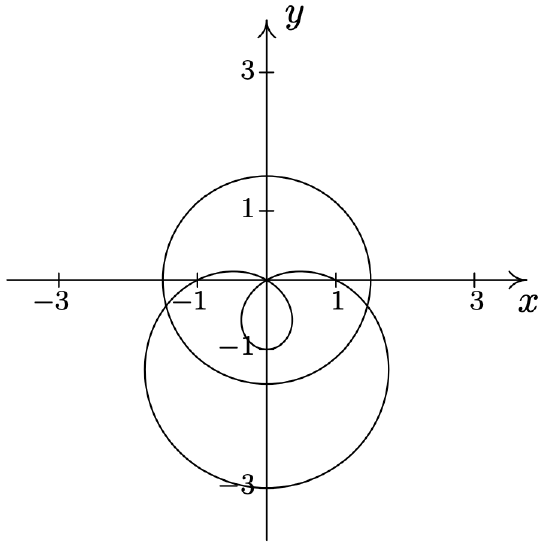
1. \(r=2 \sin (\theta) \text { and } r=2-2 \sin (\theta)\)
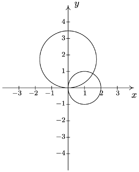
2. \(r=2 \text { and } r=3 \cos (\theta)\)
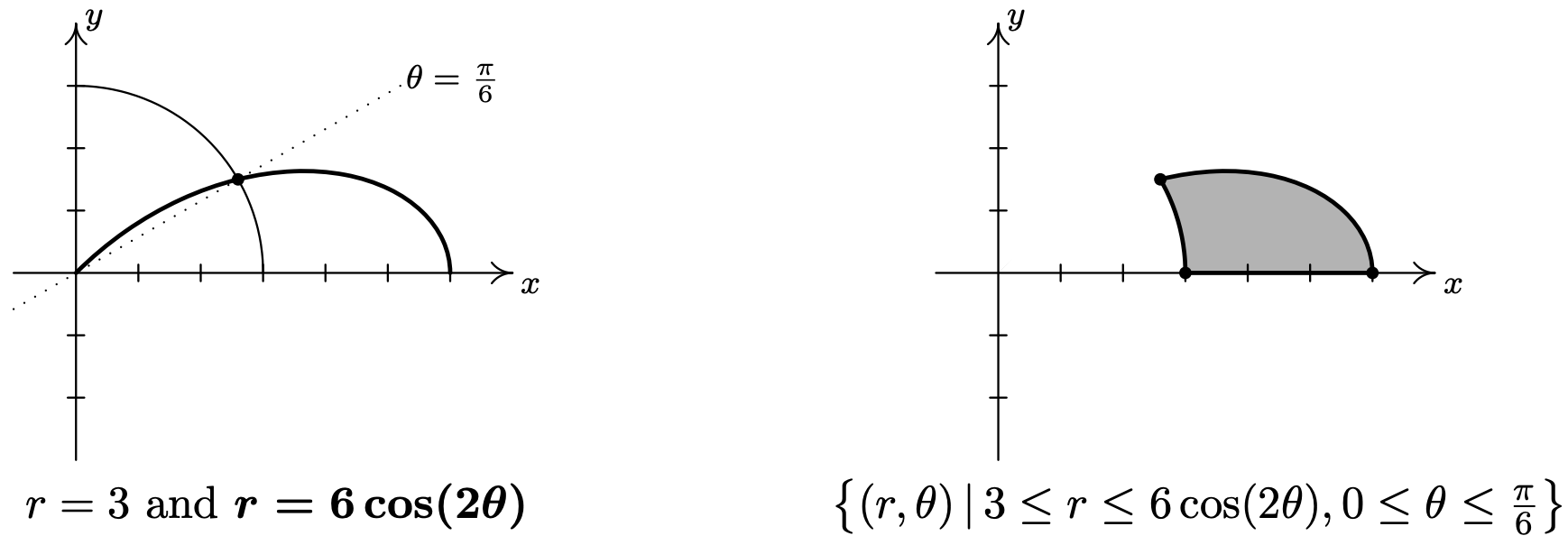
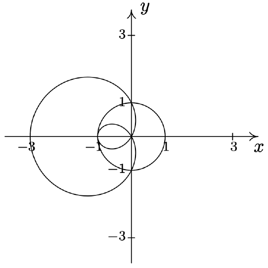
3. \(r=3 \text { and } r=6 \cos (2 \theta)\)
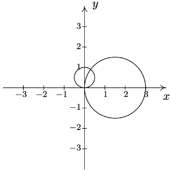
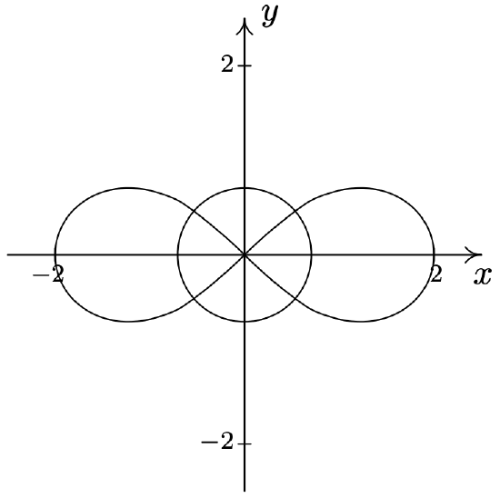
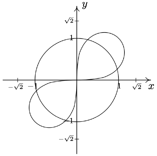
4. \(r=3 \sin \left(\frac{\theta}{2}\right) \text { and } r=3 \cos \left(\frac{\theta}{2}\right)\)

Solution

1. 
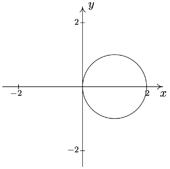
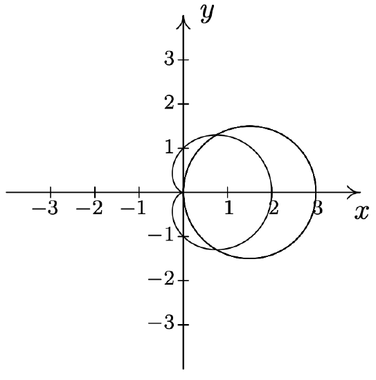
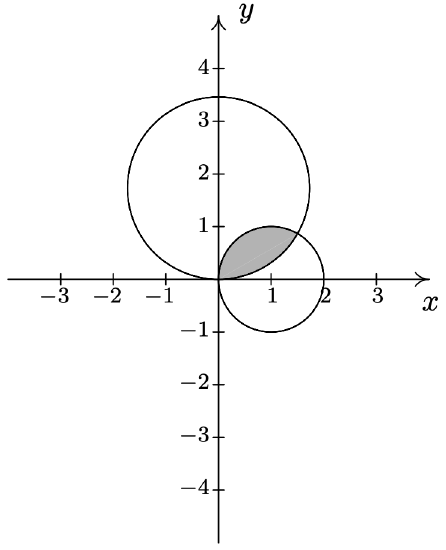
2. As before, we make a quick sketch of \(r = 2\) and \(r=3 \cos (\theta)\) to get feel for the number and location of the intersection points. The graph of \(r = 2\) is a circle, centered at the origin, with a radius of 2. The graph of \(r=3 \cos (\theta)\) is also a circle - but this one is centered at the point with rectangular coordinates \(\left(\frac{3}{2}, 0\right)\) and has a radius \(\frac{3}{2}\).

   

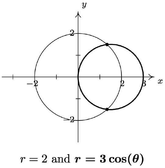
   We have two intersection points to find, one in Quadrant I and one in Quadrant IV. Proceeding as above, we first determine if any of the intersection points \(P\) have a representation \((r, \theta)\) which satisfies both \(r = 2\) and \(r=3 \cos (\theta)\). Equating these two expressions for \(r\), we get \(\cos (\theta)=\frac{2}{3}\). To solve this equation, we need the arccosine function. We get \(\theta=\arccos \left(\frac{2}{3}\right)+2 \pi k \text { or } \theta=2 \pi-\arccos \left(\frac{2}{3}\right)+2 \pi k \text { for integers } k\). From these solutions, we get \(\left(2, \arccos \left(\frac{2}{3}\right)\right)\) as one representation for our answer in Quadrant I, and \(\left(2,2 \pi-\arccos \left(\frac{2}{3}\right)\right)\) as one representation for our answer in Quadrant IV. The reader is encouraged to check these results algebraically and geometrically.

3. Proceeding as above, we first graph \(r = 3\) and \(r=6 \cos (2 \theta)\) to get an idea of how many intersection points to expect and where they lie. The graph of \(r = 3\) is a circle centered at the origin with a radius of 3 and the graph of \(r=6 \cos (2 \theta)\) is another four-leafed rose.¹² It appears as if there are eight points of intersection - two in each quadrant. We first look to see if there any points \(P(r, \theta)\) with a representation that satisfies both \(r = 3\) and \(r=6 \cos (2 \theta)\). For these points, \(6 \cos (2 \theta)=3 \text { or } \cos (2 \theta)=\frac{1}{2}\). Solving, we get \(\theta=\frac{\pi}{6}+\pi k \text { or } \theta=\frac{5 \pi}{6}+\pi k\) for integers \(k\). Out of all of these solutions, we obtain just four distinct points represented by \(\left(3, \frac{\pi}{6}\right),\left(3, \frac{5 \pi}{6}\right),\left(3, \frac{7 \pi}{6}\right) \text { and }\left(3, \frac{11 \pi}{6}\right)\). To determine the coordinates of the remaining four points, we have to consider how the representations of the points of intersection can differ. We know from Section 11.4 that if \((r, \theta) \text { and }\left(r^{\prime}, \theta^{\prime}\right)\) represent the same point and \(r \neq 0\), then either \(r=r^{\prime} \text { or } r=-r^{\prime}\). If \(r=r^{\prime}\), then \(\theta^{\prime}=\theta+2 \pi k\), so one possibility is that an intersection point \(P\) has a representation \((r, \theta)\) which satisfies \(r = 3\) and another representation \((r, \theta+2 \pi k)\) for some integer, \(k\) which satisfies \(r=6 \cos (2 \theta)\). At this point,¹³ if we replace every occurrence of \(\theta\) in the equation \(r=6 \cos (2 \theta)\) with \((\theta+2 \pi k)\) and then see if, by equating the resulting expressions for \(r\), we get any more solutions for \(\theta\). Since \(\cos (2(\theta+2 \pi k))=\cos (2 \theta+4 \pi k)=\cos (2 \theta)\) for every integer \(k\), however, the equation \(r=6 \cos (2(\theta+2 \pi k))\) reduces to the same equation we had before, \(r=6 \cos (2 \theta)\), which means we get no additional solutions. Moving on to the case where \(r=-r^{\prime}\), we have that \(\theta^{\prime}=\theta+(2 k+1) \pi\) for integers \(k\). We look to see if we can find points \(P\) which have a representation \((r, \theta)\) that satisfies \(r = 3\) and another, \((-r, \theta+(2 k+1) \pi)\), that satisfies \(r=6 \cos (2 \theta)\). To do this, we substitute¹⁴ \((-r)\) for \(r\) and \((\theta+(2 k+1) \pi)\) for \(\theta\) in the equation \(r=6 \cos (2 \theta)\) and get \(-r=6 \cos (2(\theta+(2 k+1) \pi))\). Since \(\cos (2(\theta+(2 k+1) \pi))=\cos (2 \theta+(2 k+1)(2 \pi))=\cos (2 \theta)\) for all integers \(k\), the equation \(-r=6 \cos (2(\theta+(2 k+1) \pi))\) reduces to \(-r=6 \cos (2 \theta)\), or \(r=-6 \cos (2 \theta)\). Coupling this equation with \(r = 3\) gives \(-6 \cos (2 \theta)=3\) or \(\cos (2 \theta)=-\frac{1}{2}\). We get \(\theta=\frac{\pi}{3}+\pi k \text { or } \theta=\frac{2 \pi}{3}+\pi k\). From these solutions, we obtain¹⁵ the remaining four intersection points with representations \(\left(-3, \frac{\pi}{3}\right),\left(-3, \frac{2 \pi}{3}\right),\left(-3, \frac{4 \pi}{3}\right) \text { and }\left(-3, \frac{5 \pi}{3}\right)\), which we can readily check graphically.
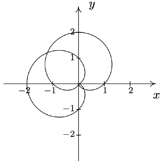
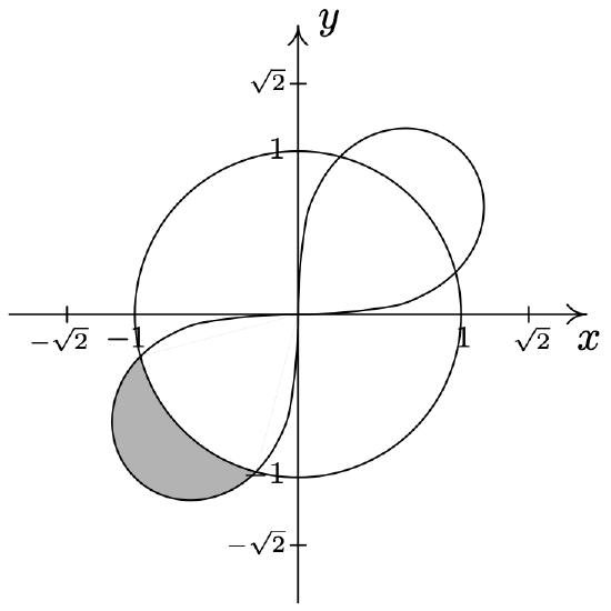
4. As usual, we begin by graphing \(r=3 \sin \left(\frac{\theta}{2}\right) \text { and } r=3 \cos \left(\frac{\theta}{2}\right)\). Using the techniques presented in Example 11.5.2, we find that we need to plot both function \(\theta\) ranges from 0 to \(4 \pi\) to obtain the complete graph. To our surprise and/or delight, it appears as if these two equations describe the same curve!

   

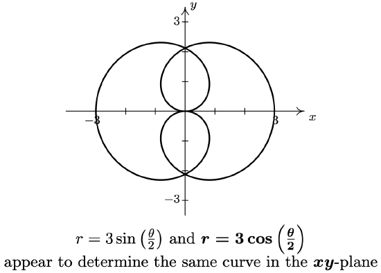
   plane To verify this incredible claim,¹⁶ we need to show that, in fact, the graphs of these two equations intersect at all points on the plane. Suppose \(P\) has a representation \((r, \theta)\) which satisfies both \(r=3 \sin \left(\frac{\theta}{2}\right) \text { and } r=3 \cos \left(\frac{\theta}{2}\right)\). Equating these two expressions for \(r\) gives the equation \(3 \sin \left(\frac{\theta}{2}\right)=3 \cos \left(\frac{\theta}{2}\right)\). While normally we discourage dividing by a variable expression (in case it could be 0), we note here that if \(3 \cos \left(\frac{\theta}{2}\right)=0\), then for our equation to hold, \(3 \sin \left(\frac{\theta}{2}\right)=0\) as well. Since no angles have both cosine and sine equal to zero, we are safe to divide both sides of the equation \(3 \sin \left(\frac{\theta}{2}\right)=3 \cos \left(\frac{\theta}{2}\right)\) by \(3 \cos \left(\frac{\theta}{2}\right)\) to get \(\tan \left(\frac{\theta}{2}\right)=1\) which gives \(\theta=\frac{\pi}{2}+2 \pi k\) for integers \(k\). From these solutions, however, we get only one intersection point which can be represented by \(\left(\frac{3 \sqrt{2}}{2}, \frac{\pi}{2}\right)\). We now investigate other representations for the intersection points. Suppose \(P\) is an intersection point with a representation \((r, \theta)\) which satisfies \(r=3 \sin \left(\frac{\theta}{2}\right)\) and the same point \(P\) has a different representation \((r, \theta+2 \pi k)\) for some integer \(k\) which satisfies \(r=3 \cos \left(\frac{\theta}{2}\right)\). Substituting into the latter, we get \(r=3 \cos \left(\frac{1}{2}[\theta+2 \pi k]\right)=3 \cos \left(\frac{\theta}{2}+\pi k\right)\). Using the sum formula for cosine, we expand \(3 \cos \left(\frac{\theta}{2}+\pi k\right)=3 \cos \left(\frac{\theta}{2}\right) \cos (\pi k)-3 \sin \left(\frac{\theta}{2}\right) \sin (\pi k)=\pm 3 \cos \left(\frac{\theta}{2}\right)\), since \(\sin (\pi k)=0\) for all integer \(k\), and \(\cos (\pi k)=\pm 1\) for all integers k. If k is an even integer, we get the same equation \(r=3 \cos \left(\frac{\theta}{2}\right)\) as before. If \(k\) is odd, we get \(r=-3 \cos \left(\frac{\theta}{2}\right)\). This latter expression for \(r\) leads to the equation \(3 \sin \left(\frac{\theta}{2}\right)=-3 \cos \left(\frac{\theta}{2}\right)\), or \(\tan \left(\frac{\theta}{2}\right)=-1\). Solving we get \(\theta=-\frac{\pi}{2}+2 \pi k\) for integers \(k\), which gives the intersection point \(\left(\frac{3 \sqrt{2}}{2},-\frac{\pi}{2}\right)\). Next, we assume \(P\) has a representation \((r, \theta)\) which satisfies \(r=3 \sin \left(\frac{\theta}{2}\right)\) and a representation \((-r, \theta+(2 k+1) \pi)\) which satisfies \(r=3 \cos \left(\frac{\theta}{2}\right)\) for some integer \(k\). Substituting \((-r)\) for \(r\) and \((\theta+(2 k+1) \pi)\) in for \(\theta\) into \(r=3 \cos \left(\frac{\theta}{2}\right)\) gives \(-r=3 \cos \left(\frac{1}{2}[\theta+(2 k+1) \pi]\right)\). Once again, we use the sum formula for cosine to get

   \(\begin{aligned}
   \cos \left(\frac{1}{2}[\theta+(2 k+1) \pi]\right) &=\cos \left(\frac{\theta}{2}+\frac{(2 k+1) \pi}{2}\right) \\
   &=\cos \left(\frac{\theta}{2}\right) \cos \left(\frac{(2 k+1) \pi}{2}\right)-\sin \left(\frac{\theta}{2}\right) \sin \left(\frac{(2 k+1) \pi}{2}\right) \\
   &=\pm \sin \left(\frac{\theta}{2}\right)
   \end{aligned}\)

   where the last equality is true since \(\cos\left(\frac{(2 k+1) \pi}{2}\right)=0\) and \(\sin \left(\frac{(2 k+1) \pi}{2}\right)=\pm 1\) for integers \(k\). Hence, \(-r=3 \cos \left(\frac{1}{2}[\theta+(2 k+1) \pi]\right)\) can be rewritten as \(r=\pm 3 \sin \left(\frac{\theta}{2}\right)\). If we choose \(k=0\), then \(\sin \left(\frac{(2 k+1) \pi}{2}\right)=\sin \left(\frac{\pi}{2}\right)=1\), and the equation \(-r=3 \cos \left(\frac{1}{2}[\theta+(2 k+1) \pi]\right)\) in this case reduces to \(-r=-3 \sin \left(\frac{\theta}{2}\right)\), or \(r=3 \sin \left(\frac{\theta}{2}\right)\) which is the other equation under consideration! What this means is that if a polar representation \((r, \theta)\) for the point \(P\) satisfies \(r=3 \sin \left(\frac{\theta}{2}\right)\), then the representation \((-r, \theta+\pi)\) for \(P\) automatically satisfies \(r=3 \cos \left(\frac{\theta}{2}\right)\). Hence the equations \(r=3 \sin \left(\frac{\theta}{2}\right)\) and \(r=3 \cos \left(\frac{\theta}{2}\right)\) determine the same set of points in the plane.

Our work in Example 11.5.3 justifies the following.

Guidelines for Finding Points of Intersection of Graphs of Polar Equations

To find the points of intersection of the graphs of two polar equations \(E_{1}\) and \(E_{2}\):

• Sketch the graphs of \(E_{1}\) and \(E_{2}\). Check to see if the curves intersect at the origin (pole).
• Solve for pairs \((r, \theta)\) which satisfy both \(E_{1}\) and \(E_{2}\).
• substitute \((\theta+2 \pi k)\) for \(\theta\) in either one of \(E_{1}\) or \(E_{2}\) (but not both) and solve for pairs \((r, \theta)\) which satisfy both equations. Keep in mind that \(k\) is an integer.
• Substitute \((-r)\) for \(r\) and \((\theta+(2 k+1) \pi)\) for \(\theta\) in either one of \(E_{1}\) or \(E_{2}\) (but not both) and solve for pairs \((r, \theta)\) which satisfy both equations. Keep in mind that \(k\) is an integer.

Our last example ties together graphing and points of intersection to describe regions in the plane.

Example 11.5.4

Sketch the region in the \(xy\)-plane described by the following sets.

1. \(\left\{(r, \theta) \mid 0 \leq r \leq 5 \sin (2 \theta), 0 \leq \theta \leq \frac{\pi}{2}\right\}\)
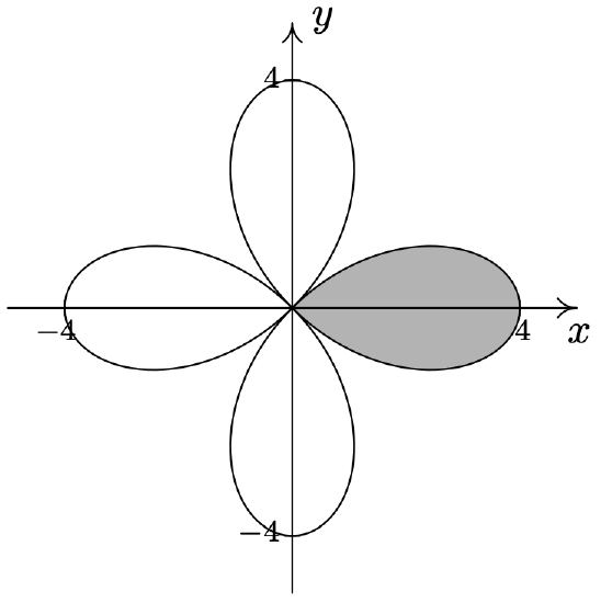
2. \(\left\{(r, \theta) \mid 3 \leq r \leq 6 \cos (2 \theta), 0 \leq \theta \leq \frac{\pi}{6}\right\}\)
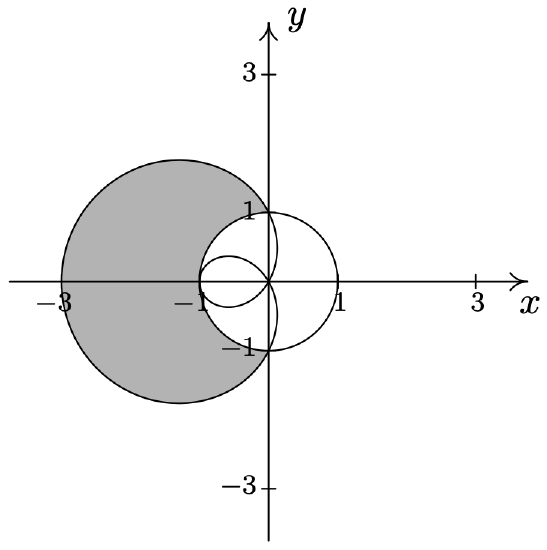
3. \(\left\{(r, \theta) \mid 2+4 \cos (\theta) \leq r \leq 0, \frac{2 \pi}{3} \leq \theta \leq \frac{4 \pi}{3}\right\}\)
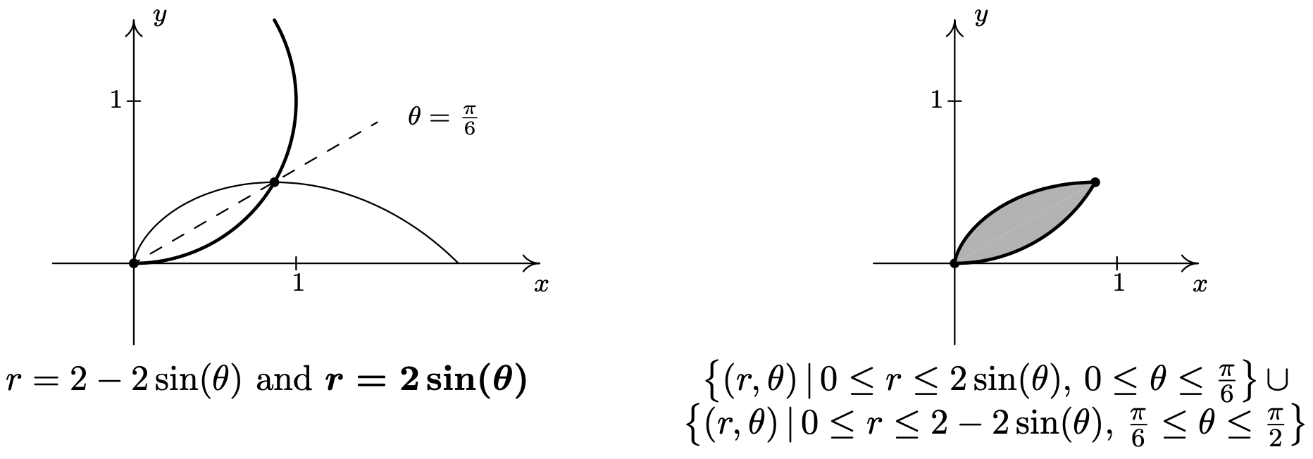
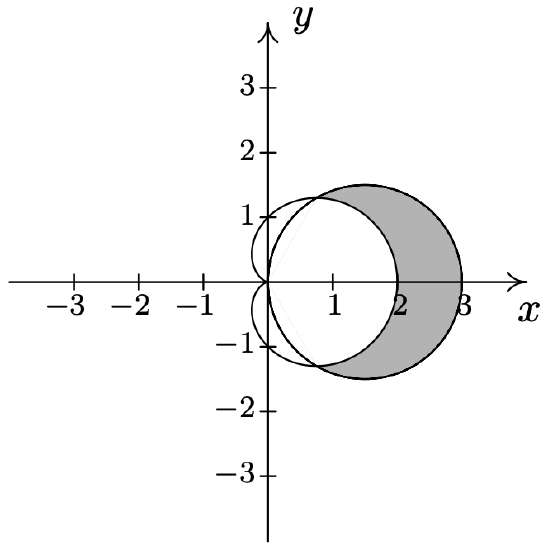
4. \(\left\{(r, \theta) \mid 0 \leq r \leq 2 \sin (\theta), 0 \leq \theta \leq \frac{\pi}{6}\right\} \cup\left\{(r, \theta) \mid 0 \leq r \leq 2-2 \sin (\theta), \frac{\pi}{6} \leq \theta \leq \frac{\pi}{2}\right\}\)

Solution

Our first step in these problems is to sketch the graphs of the polar equations involved to get a sense of the geometric situation. Since all of the equations in this example are found in either Example 11.5.2 or Example 11.5.3, most of the work is done for us.

1. We know from Example 11.5.2 number 3 that the graph of \(r=5 \sin (2 \theta)\) is a rose. Moreover, we know from our work there that as \(0 \leq \theta \leq \frac{\pi}{2}\), we are tracing out the ‘leaf’ of the rose which lies in the first quadrant. The inequality \(0 \leq r \leq 5 \sin (2 \theta)\) means we want to capture all of the points between the origin \((r = 0)\) and the curve \(r=5 \sin (2 \theta)\) as \(\theta\) runs through \(\left[0, \frac{\pi}{2}\right]\). Hence, the region we seek is the leaf itself.

   

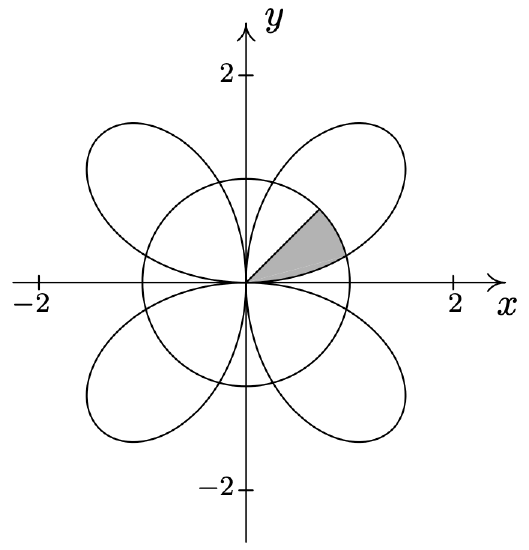
2. We know from Example 11.5.3 number 3 that \(r = 3\) and \(r=6 \cos (2 \theta)\) intersect at \(\theta=\frac{\pi}{6}\), so the region that is being described here is the set of points whose directed distance \(r\) from the origin is at least 3 but no more than \(6 \cos (2 \theta)\) as \(\theta\) runs from 0 to \(\frac{\pi}{6}\). In other words, we are looking at the points outside or on the circle (since \(r \geq 3\)) but inside or on the rose (since \(r \leq 6 \cos (2 \theta)\)). We shade the region below.

   

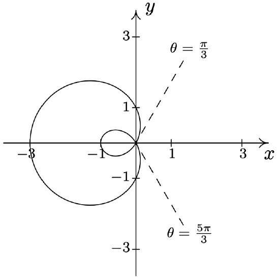
3. From Example 11.5.2 number 2, we know that the graph of \(r=2+4 \cos (\theta)\) is a limaçon whose ‘inner loop’ is traced out as \(\theta\) runs through the given values \(\frac{2 \pi}{3}\) to \(\frac{4 \pi}{3}\). Since the values \(r\) takes on in this interval are non-positive, the inequality \(2+4 \cos (\theta) \leq r \leq 0\) makes sense, and we are looking for all of the points between the pole \(r = 0\) and the limaçon as \(\theta\) ranges over the interval \(\left[\frac{2 \pi}{3}, \frac{4 \pi}{3}\right]\). In other words, we shade in the inner loop of the limaçon.

   

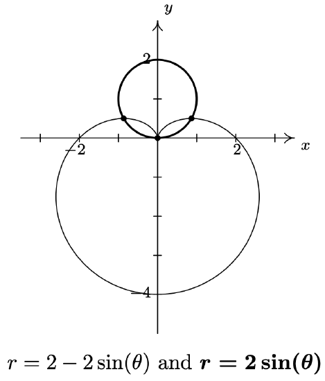
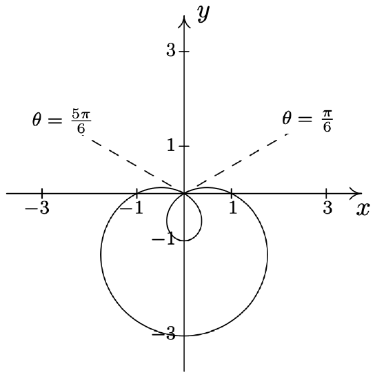
4. We have two regions described here connected with the union symbol \(\text { 'U.' }\) We shade each in turn and find our final answer by combining the two. In Example 11.5.3, number 1, we found that the curves \(r=2 \sin (\theta)\) and \(r=2-2 \sin (\theta)\) intersect when \(\theta=\frac{\pi}{6}\). Hence, for the first region, \(\left\{(r, \theta) \mid 0 \leq r \leq 2 \sin (\theta), 0 \leq \theta \leq \frac{\pi}{6}\right\}\), we are shading the region between the origin \((r = 0)\) out to the circle \((r=2 \sin (\theta))\) as \(\theta\) ranges from 0 to \(\frac{\pi}{6}\), which is the angle of intersection of the two curves. For the second region, \(\left\{(r, \theta) \mid 0 \leq r \leq 2-2 \sin (\theta), \frac{\pi}{6} \leq \theta \leq \frac{\pi}{2}\right\}\), \(\theta\) picks up where it left off at \(\frac{\pi}{6}\) and continues to \(\frac{\pi}{2}\). In this case, however, we are shading from the origin \((r = 0)\) out to the cardioid \(r=2-2 \sin (\theta)\) which pulls into the origin at \(\theta=\frac{\pi}{2}\). Putting these two regions together gives us our final answer.

   

11.5.1 Exercises

In Exercises 1 - 20, plot the graph of the polar equation by hand. Carefully label your graphs.

1. \(\text { Circle: } r=6 \sin (\theta)\)
2. \(\text { Circle: } r=2 \cos (\theta)\)
3. \(\text { Rose: } r=2 \sin (2 \theta)\)
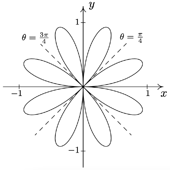
4. \(\text { Rose: } r=4 \cos (2 \theta)\)
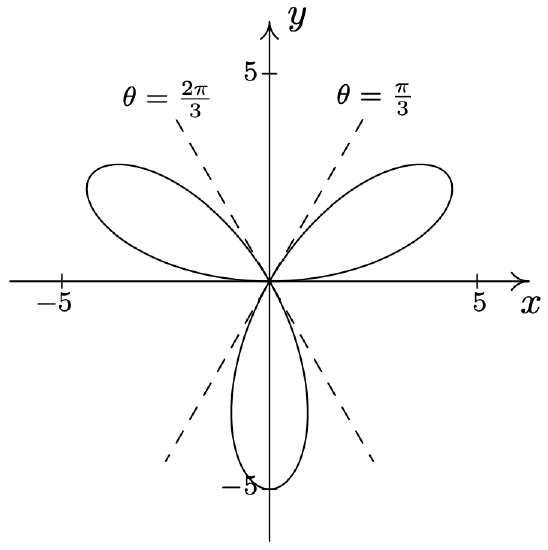
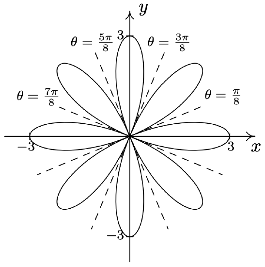
5. \(\text { Rose: } r=5 \sin (3 \theta)\)
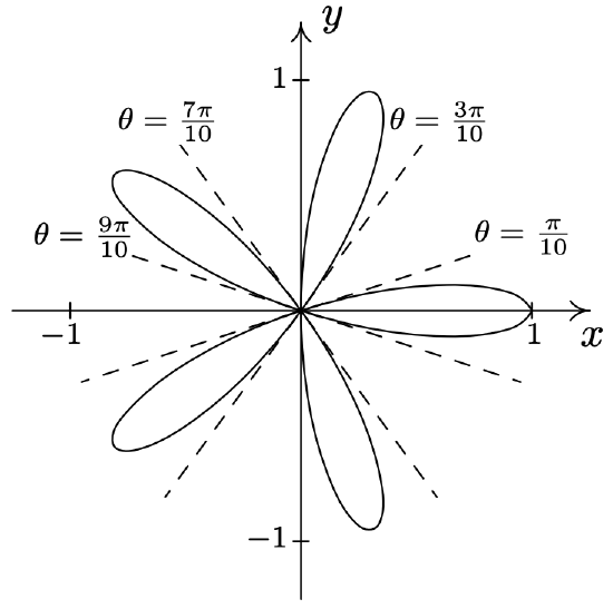
6. \(\text { Rose: } r=\cos (5 \theta)\)
7. \(\text { Rose: } r=\sin (4 \theta)\)
8. \(\text { Rose: } r=3 \cos (4 \theta)\)
9. \(\text { Cardioid: } r=3-3 \cos (\theta)\)
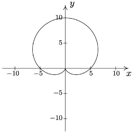
10. \(\text { Cardioid: } r=5+5 \sin (\theta)\)
11. \(\text { Cardioid: } r=2+2 \cos (\theta)\)
12. \(\text { Cardioid: } r=1-\sin (\theta)\)
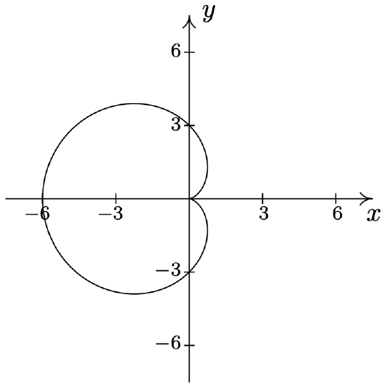
13. \(\text { Limaçon: } r=1-2 \cos (\theta)\)
14. \(\text { Limaçon: } r=1-2 \sin (\theta)\)
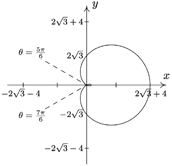
15. \(\text { Limaçon: } r=2 \sqrt{3}+4 \cos (\theta)\)
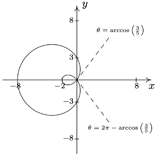
16. \(\text { Limaçon: } r=3-5 \cos (\theta)\)
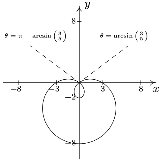
17. \(\text { Limaçon: } r=3-5 \sin (\theta)\)
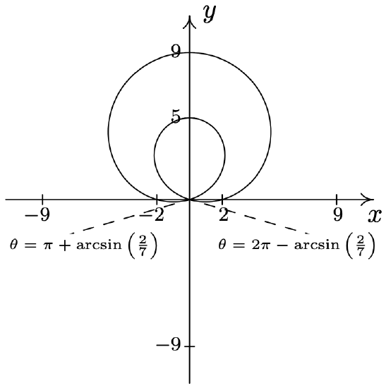
18. \(\text { Limaçon: } r=2+7 \sin (\theta)\)
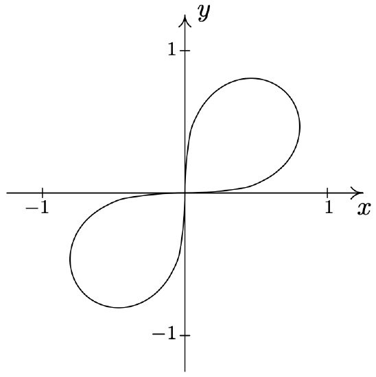
19. \(\text { Lemniscate: } r^{2}=\sin (2 \theta)\)
20. \(\text { Lemniscate: } r^{2}=4 \cos (2 \theta)\)

In Exercises 21 - 30, find the exact polar coordinates of the points of intersection of graphs of the polar equations. Remember to check for intersection at the pole (origin).

21. \(r=3 \cos (\theta) \text { and } r=1+\cos (\theta)\)
22. \(r=1+\sin (\theta) \text { and } r=1-\cos (\theta)\)
23. \(r=1-2 \sin (\theta) \text { and } r=2\)
24. \(r=1-2 \cos (\theta) \text { and } r=1\)
25. \(r=2 \cos (\theta) \text { and } r=2 \sqrt{3} \sin (\theta)\)
26. \(r=3 \cos (\theta) \text { and } r=\sin (\theta)\)
27. \(r^{2}=4 \cos (2 \theta) \text { and } r=\sqrt{2}\)
28. \(r^{2}=2 \sin (2 \theta) \text { and } r=1\)
29. \(r=4 \cos (2 \theta) \text { and } r=2\)
30. \(r=2 \sin (2 \theta) \text { and } r=1\)

In Exercises 31 - 40, sketch the region in the \(xy\)-plane described by the given set.

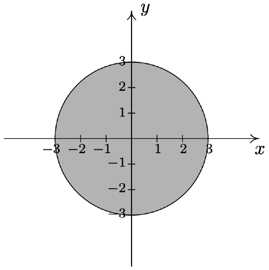
31. \(\{(r, \theta) \mid 0 \leq r \leq 3,0 \leq \theta \leq 2 \pi\}\)
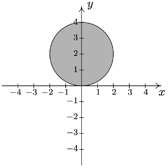
32. \(\{(r, \theta) \mid 0 \leq r \leq 4 \sin (\theta), 0 \leq \theta \leq \pi\}\)
33. \(\left\{(r, \theta) \mid 0 \leq r \leq 3 \cos (\theta),-\frac{\pi}{2} \leq \theta \leq \frac{\pi}{2}\right\}\)
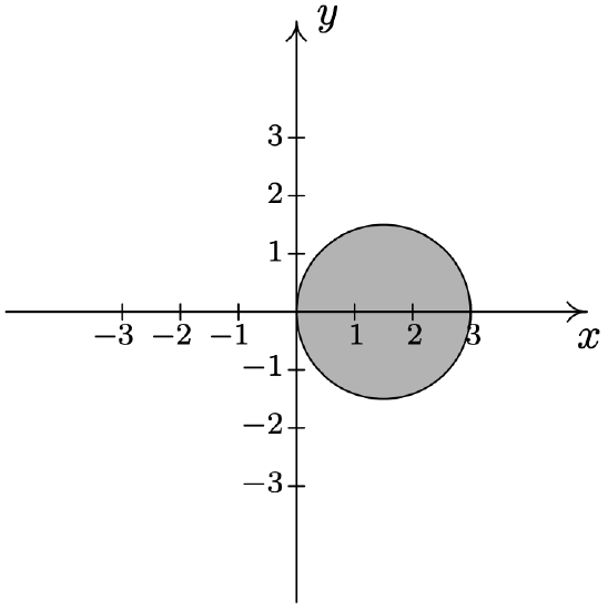
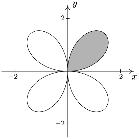
34. \(\left\{(r, \theta) \mid 0 \leq r \leq 2 \sin (2 \theta), 0 \leq \theta \leq \frac{\pi}{2}\right\}\)
35. \(\left\{(r, \theta) \mid 0 \leq r \leq 4 \cos (2 \theta),-\frac{\pi}{4} \leq \theta \leq \frac{\pi}{4}\right\}\)
36. \(\left\{(r, \theta) \mid 1 \leq r \leq 1-2 \cos (\theta), \frac{\pi}{2} \leq \theta \leq \frac{3 \pi}{2}\right\}\)
37. \(\left\{(r, \theta) \mid 1+\cos (\theta) \leq r \leq 3 \cos (\theta),-\frac{\pi}{3} \leq \theta \leq \frac{\pi}{3}\right\}\)
38. \(\left\{(r, \theta) \mid 1 \leq r \leq \sqrt{2 \sin (2 \theta)}, \frac{13 \pi}{12} \leq \theta \leq \frac{17 \pi}{12}\right\}\)
39. \(\left\{(r, \theta) \mid 0 \leq r \leq 2 \sqrt{3} \sin (\theta), 0 \leq \theta \leq \frac{\pi}{6}\right\} \cup\left\{(r, \theta) \mid 0 \leq r \leq 2 \cos (\theta), \frac{\pi}{6} \leq \theta \leq \frac{\pi}{2}\right\}\)
40. \(\left\{(r, \theta) \mid 0 \leq r \leq 2 \sin (2 \theta), 0 \leq \theta \leq \frac{\pi}{12}\right\} \cup\left\{(r, \theta) \mid 0 \leq r \leq 1, \frac{\pi}{12} \leq \theta \leq \frac{\pi}{4}\right\}\)

In Exercises 41 - 50, use set-builder notation to describe the polar region. Assume that the region contains its bounding curves.

41. The region inside the circle \(r = 5\).
42. The region inside the circle \(r = 5\) which lies in Quadrant III.
43. The region inside the left half of the circle \(r=6 \sin (\theta)\).
44. The region inside the circle \(r=4 \cos (\theta)\) which lies in Quadrant IV.
45. The region inside the top half of the cardioid \(r=3-3 \cos (\theta)\)
46. The region inside the cardioid \(r=2-2 \sin (\theta)\) which lies in Quadrants I and IV.
47. The inside of the petal of the rose \(r=3 \cos (4 \theta)\) which lies on the positive \(x\)-axis
48. The region inside the circle \(r = 5\) but outside the circle \(r = 3\).
49. The region which lies inside of the circle \(r=3 \cos (\theta)\) but outside of the circle \(r=\sin (\theta)\)
50. The region in Quadrant I which lies inside both the circle \(r = 3\) as well as the rose \(r=6 \sin (2 \theta)\)

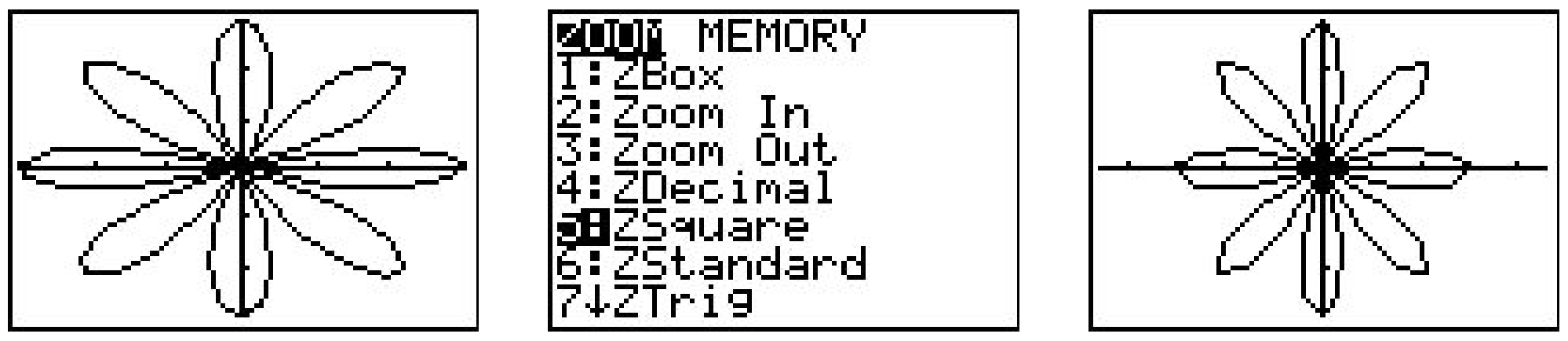
While the authors truly believe that graphing polar curves by hand is fundamental to your understanding of the polar coordinate system, we would be derelict in our duties if we totally ignored the graphing calculator. Indeed, there are some important polar curves which are simply too difficult to graph by hand and that makes the calculator an important tool for your further studies in Mathematics, Science and Engineering. We now give a brief demonstration of how to use the graphing calculator to plot polar curves. The first thing you must do is switch the MODE of your calculator to POL, which stands for “polar”.

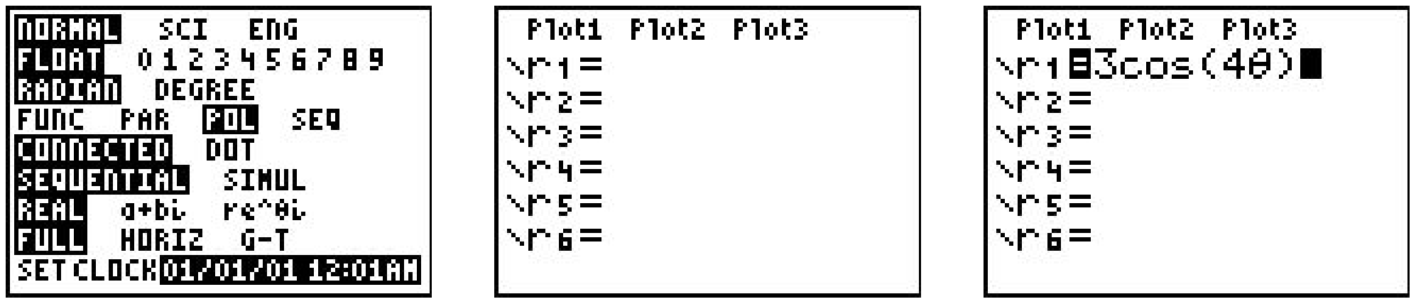
This changes the \(\text { " } Y="\) menu as seen above in the middle. Let’s plot the polar rose given by \(r=3 \cos (4 \theta)\) from Exercise 8 above. We type the function into the “r=” menu as seen above on the right. We need to set the viewing window so that the curve displays properly, but when we look at the WINDOW menu, we find three extra lines.

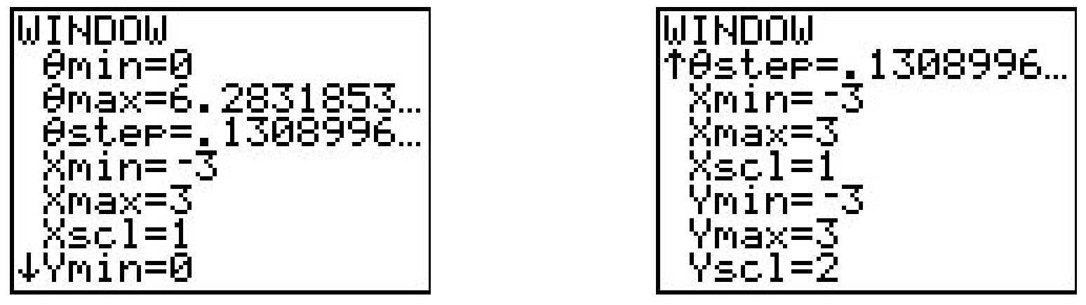
In order for the calculator to be able to plot \(r=3 \cos (4 \theta)\) in the \(xy\)-plane, we need to tell it not only the dimensions which \(x\) and \(y\) will assume, but we also what values of \(\theta\) to use. From our previous work, we know that we need \(0 \leq \theta \leq 2 \pi\), so we enter the data you see above. (I’ll say more about the \(\theta \text {-step }\) in just a moment.) Hitting GRAPH yields the curve below on the left which doesn’t look quite right. The issue here is that the calculator screen is 96 pixels wide but only 64 pixels tall. To get a true geometric perspective, we need to hit ZOOM SQUARE (seen below in the middle) to produce a more accurate graph which we present below on the right.

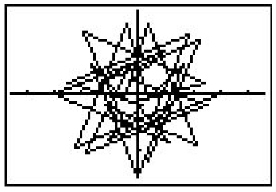
In function mode, the calculator automatically divided the interval [Xmin, Xmax] into 96 equal subintervals. In polar mode, however, we must specify how to split up the interval \([\theta \min , \theta \max ]\) using the \(\theta \text {step}\). For most graphs, a \(\theta \text {step}\) of 0.1 is fine. If you make it too small then the calculator takes a long time to graph. It you make it too big, you get chunky garbage like this.

You will need to experiment with the settings in order to get a nice graph. Exercises 51 - 60 give you some curves to graph using your calculator. Notice that some of them have explicit bounds on \(\theta\) and others do not.

51. \(r=\theta, 0 \leq \theta \leq 12 \pi\)
52. \(r=\ln (\theta), 1 \leq \theta \leq 12 \pi\)
53. \(r=e^{.1 \theta}, 0 \leq \theta \leq 12 \pi\)
54. \(r=\theta^{3}-\theta,-1.2 \leq \theta \leq 1.2\)
55. \(r=\sin (5 \theta)-3 \cos (\theta)\)
56. \(r=\sin ^{3}\left(\frac{\theta}{2}\right)+\cos ^{2}\left(\frac{\theta}{3}\right)\)
57. \(r=\arctan (\theta),-\pi \leq \theta \leq \pi\)
58. \(r=\frac{1}{1-\cos (\theta)}\)
59. \(r=\frac{1}{2-\cos (\theta)}\)
60. \(r=\frac{1}{2-3 \cos (\theta)}\)
61. How many petals does the polar rose \(r=\sin (2 \theta)\) ) have? What about \(r=\sin (3 \theta), r=\sin (4 \theta)\) and \(r=\sin (5 \theta)\)? ? With the help of your classmates, make a conjecture as to how many petals the polar rose \(r=\sin (n \theta)\) ) has for any natural number \(n\). Replace sine with cosine and repeat the investigation. How many petals does \(r=\cos (n \theta)\) have for each natural number \(n\)?

Looking back through the graphs in the section, it’s clear that many polar curves enjoy various forms of symmetry. However, classifying symmetry for polar curves is not as straight-forward as it was for equations back on page 26. In Exercises 62 - 64, we have you and your classmates explore some of the more basic forms of symmetry seen in common polar curves.

62. Show that if \(f\) is even¹⁷ then the graph of \(r=f(\theta)\) is symmetric about the \(x\)-axis.
    1. Show that \(f(\theta)=2+4 \cos (\theta)\) is even and verify that the graph of \(r=2+4 \cos (\theta)\) is indeed symmetric about the \(x\)-axis. (See Example 11.5.2 number 2.)
    2. Show that \(f(\theta)=3 \sin \left(\frac{\theta}{2}\right)\) is not even, yet the graph of \(r=3 \sin \left(\frac{\theta}{2}\right)\) is symmetric about the \(x\)-axis. (See Example 11.5.3 number 4.)
63. Show that if \(f\) is odd¹⁸ then the graph of \(r=f(\theta)\) is symmetric about the origin.
    1. Show that \(f(\theta)=5 \sin (2 \theta)\) is odd and verify that the graph of \(r=5 \sin (2 \theta)\) is indeed symmetric about the origin. (See Example 11.5.2 number 3.)
    2. Show that \(f(\theta)=3 \cos \left(\frac{\theta}{2}\right)\) is not odd, yet the graph of \(r=3 \cos \left(\frac{\theta}{2}\right)\) is symmetric about the origin. (See Example 11.5.3 number 4.)
64. Show that if \(f(\pi-\theta)=f(\theta)\) for all \(\theta\) in the domain of \(f\) then the graph of \(r=f(\theta)\) is symmetric about the \(y\)-axis.
    1. For \(f(\theta)=4-2 \sin (\theta)\), show that \(f(\pi-\theta)=f(\theta)\) and the graph of \(r=4-2 \sin (\theta)\) is symmetric about the \(y\)-axis, as required. (See Example 11.5.2 number 1.)
    2. For \(f(\theta)=5 \sin (2 \theta)\), show that \(f\left(\pi-\frac{\pi}{4}\right) \neq f\left(\frac{\pi}{4}\right)\), yet the graph of \(r=5 \sin (2 \theta)\) is symmetric about the \(y\)-axis. (See Example 11.5.2 number 3.)

In Section 1.7, we discussed transformations of graphs. In Exercise 65 we have you and your classmates explore transformations of polar graphs.

65. For Exercises 65a and 65b below, let \(f(\theta)=\cos (\theta) \text { and } g(\theta)=2-\sin (\theta)\).
    1. Using your graphing calculator, compare the graph of \(r=f(\theta)\) to each of the graphs of \(r=f\left(\theta+\frac{\pi}{4}\right), r=f\left(\theta+\frac{3 \pi}{4}\right), r=f\left(\theta-\frac{\pi}{4}\right) \text { and } r=f\left(\theta-\frac{3 \pi}{4}\right)\). Repeat this process for \(g(\theta)\). In general, how do you think the graph of \(r=f(\theta+\alpha)\) compares with the graph of \(r=f(\theta)\)?
    2. Using your graphing calculator, compare the graph of \(r=f(\theta)\) to each of the graphs of \(r=2 f(\theta), r=\frac{1}{2} f(\theta), r=-f(\theta) \text { and } r=-3 f(\theta)\). Repeat this process for \(g(\theta)\). In general, how do you think the graph of \(r=k \cdot f(\theta)\) compares with the graph of \(r=f(\theta)\)? (Does it matter if \(k>0\) or \(k<0\)?)
66. In light of Exercises 62 - 64, how would the graph of \(r=f(-\theta)\) compare with the graph of \(r=f(\theta)\) for a generic function \(f\)? What about the graphs of \(r=-f(\theta) \text { and } r=f(\theta)\)? What about \(r=f(\theta) \text { and } r=f(\pi-\theta)\)? Test out your conjectures using a variety of polar functions found in this section with the help of a graphing utility.
67. With the help of your classmates, research cardioid microphones.
68. Back in Section 1.2, in the paragraph before Exercise 53, we gave you this link to a fascinating list of curves. Some of these curves have polar representations which we invite you and your classmates to research.

11.5.2 Answers

1. \(\text { Circle: } r=6 \sin (\theta)\)

   

2. \(\text { Circle: } r=2 \cos (\theta)\)

   

3. \(\text { Rose: } r=2 \sin (2 \theta)\)

   

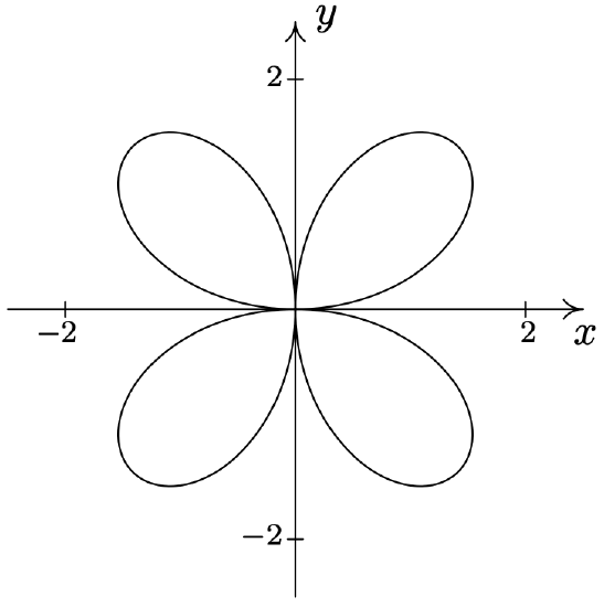
4. \(\text { Rose: } r=4 \cos (2 \theta)\)

   

5. \(\text { Rose: } r=5 \sin (3 \theta)\)

   

6. \(\text { Rose: } r=\cos (5 \theta)\)

   

7. \(\text { Rose: } r=\sin (4 \theta)\)

   

8. \(\text { Rose: } r=3 \cos (4 \theta)\)

   

9. \(\text { Cardioid: } r=3-3 \cos (\theta)\)

   

10. \(\text { Cardioid: } r=5+5 \sin (\theta)\)

    

11. \(\text { Cardioid: } r=2+2 \cos (\theta)\)

    

12. \(\text { Cardioid: } r=1-\sin (\theta)\)

    

13. \(\text { Limaçon: } r=1-2 \cos (\theta)\)

    

14. \(\text { Limaçon: } r=1-2 \sin (\theta)\)

    

15. \(\text { Limaçon: } r=2 \sqrt{3}+4 \cos (\theta)\)

    

16. \(\text { Limaçon: } r=3-5 \cos (\theta)\)

    

17. \(\text { Limaçon: } r=3-5 \sin (\theta)\)

    

18. \(\text { Limaçon: } r=2+7 \sin (\theta)\)

    

19. \(\text { Lemniscate: } r^{2}=\sin (2 \theta)\)

    

20. \(\text { Lemniscate: } r^{2}=4 \cos (2 \theta)\)

    

21. \(r=3 \cos (\theta) \text { and } r=1+\cos (\theta)\) \(\quad\quad\quad\quad\) \(\left(\frac{3}{2}, \frac{\pi}{3}\right),\left(\frac{3}{2}, \frac{5 \pi}{3}\right), \text { pole }\)

    

22. \(r=1+\sin (\theta) \text { and } r=1-\cos (\theta)\) \(\quad\quad\quad\quad\) \(\left(\frac{2+\sqrt{2}}{2}, \frac{3 \pi}{4}\right),\left(\frac{2-\sqrt{2}}{2}, \frac{7 \pi}{4}\right), \text { pole }\)

    

23. \(r=1-2 \sin (\theta) \text { and } r=2\) \(\quad\quad\quad\quad\) \(\left(2, \frac{7 \pi}{6}\right),\left(2, \frac{11 \pi}{6}\right)\)

    

24. \(r=1-2 \cos (\theta) \text { and } r=1\) \(\quad\quad\quad\quad\) \(\left(1, \frac{\pi}{2}\right),\left(1, \frac{3 \pi}{2}\right),(-1,0)\)

    

25. \(r=2 \cos (\theta) \text { and } r=2 \sqrt{3} \sin (\theta)\) \(\quad\quad\quad\quad\) \(\left(\sqrt{3}, \frac{\pi}{6}\right), \text { pole }\)

    

26. \(r=3 \cos (\theta) \text { and } r=\sin (\theta)\) \(\quad\quad\quad\quad\) \(\left(\frac{3 \sqrt{10}}{10}, \arctan (3)\right), \text { pole }\)

    

27. \(r^{2}=4 \cos (2 \theta) \text { and } r=\sqrt{2}\) \(\quad\quad\quad\quad\) \(\left(\sqrt{2}, \frac{\pi}{6}\right),\left(\sqrt{2}, \frac{5 \pi}{6}\right),\left(\sqrt{2}, \frac{7 \pi}{6}\right),\left(\sqrt{2}, \frac{11 \pi}{6}\right)\)

    

28. \(r^{2}=2 \sin (2 \theta) \text { and } r=1\) \(\quad\quad\quad\quad\) \(\left(1, \frac{\pi}{12}\right),\left(1, \frac{5 \pi}{12}\right),\left(1, \frac{13 \pi}{12}\right),\left(1, \frac{17 \pi}{12}\right)\)

    

29. \(r=4 \cos (2 \theta) \text { and } r=2\) \(\quad\quad\quad\quad\) \(\begin{aligned}
    &\left(2, \frac{\pi}{6}\right),\left(2, \frac{5 \pi}{6}\right),\left(2, \frac{7 \pi}{6}\right), \\
    &\left(2, \frac{11 \pi}{6}\right),\left(-2, \frac{\pi}{3}\right),\left(-2, \frac{2 \pi}{3}\right), \\
    &\left(-2, \frac{4 \pi}{3}\right),\left(-2, \frac{5 \pi}{3}\right) \end{aligned}\)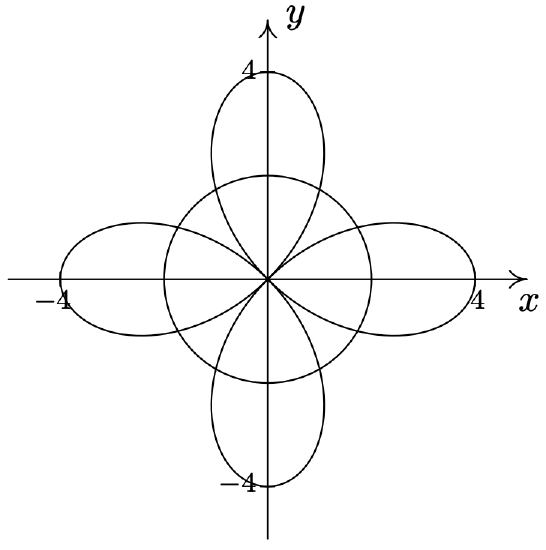

    

30. \(r=2 \sin (2 \theta) \text { and } r=1\) \(\quad\quad\quad\quad\) \(\begin{aligned}
    &\left(1, \frac{\pi}{12}\right),\left(1, \frac{5 \pi}{12}\right),\left(1, \frac{13 \pi}{12}\right), \\
    &\left(1, \frac{17 \pi}{12}\right),\left(-1, \frac{7 \pi}{12}\right),\left(-1, \frac{11 \pi}{12}\right), \\
    &\left(-1, \frac{19 \pi}{12}\right),\left(-1, \frac{23 \pi}{12}\right) \end{aligned}\)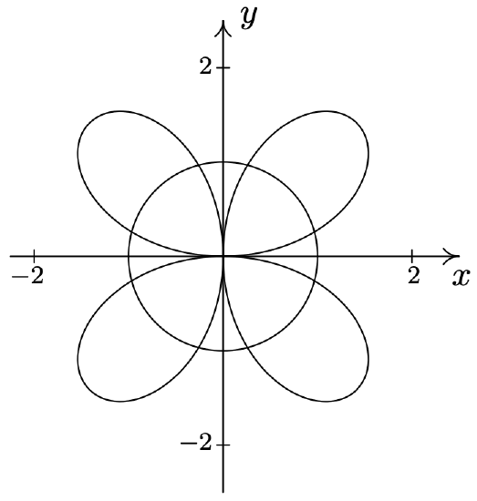

    

31. \(\{(r, \theta) \mid 0 \leq r \leq 3,0 \leq \theta \leq 2 \pi\}\)

    

32. \(\{(r, \theta) \mid 0 \leq r \leq 4 \sin (\theta), 0 \leq \theta \leq \pi\}\)

    

33. \(\left\{(r, \theta) \mid 0 \leq r \leq 3 \cos (\theta),-\frac{\pi}{2} \leq \theta \leq \frac{\pi}{2}\right\}\)

    

34. \(\left\{(r, \theta) \mid 0 \leq r \leq 2 \sin (2 \theta), 0 \leq \theta \leq \frac{\pi}{2}\right\}\)

    

35. \(\left\{(r, \theta) \mid 0 \leq r \leq 4 \cos (2 \theta),-\frac{\pi}{4} \leq \theta \leq \frac{\pi}{4}\right\}\)

    

36. \(\left\{(r, \theta) \mid 1 \leq r \leq 1-2 \cos (\theta), \frac{\pi}{2} \leq \theta \leq \frac{3 \pi}{2}\right\}\)

    

37. \(\left\{(r, \theta) \mid 1+\cos (\theta) \leq r \leq 3 \cos (\theta),-\frac{\pi}{3} \leq \theta \leq \frac{\pi}{3}\right\}\)

    

38. \(\left\{(r, \theta) \mid 1 \leq r \leq \sqrt{2 \sin (2 \theta)}, \frac{13 \pi}{12} \leq \theta \leq \frac{17 \pi}{12}\right\}\)

    

39. \(\left\{(r, \theta) \mid 0 \leq r \leq 2 \sqrt{3} \sin (\theta), 0 \leq \theta \leq \frac{\pi}{6}\right\} \cup\left\{(r, \theta) \mid 0 \leq r \leq 2 \cos (\theta), \frac{\pi}{6} \leq \theta \leq \frac{\pi}{2}\right\}\)

    

40. \(\left\{(r, \theta) \mid 0 \leq r \leq 2 \sin (2 \theta), 0 \leq \theta \leq \frac{\pi}{12}\right\} \cup\left\{(r, \theta) \mid 0 \leq r \leq 1, \frac{\pi}{12} \leq \theta \leq \frac{\pi}{4}\right\}\)

    

41. \(\{(r, \theta) \mid 0 \leq r \leq 5,0 \leq \theta \leq 2 \pi\}\)
42. \(\left\{(r, \theta) \mid 0 \leq r \leq 5, \pi \leq \theta \leq \frac{3 \pi}{2}\right\}\)
43. \(\left\{(r, \theta) \mid 0 \leq r \leq 6 \sin (\theta), \frac{\pi}{2} \leq \theta \leq \pi\right\}\)
44. \(\left\{(r, \theta) \mid 4 \cos (\theta) \leq r \leq 0, \frac{\pi}{2} \leq \theta \leq \pi\right\}\)
45. \(\{(r, \theta) \mid 0 \leq r \leq 3-3 \cos (\theta), 0 \leq \theta \leq \pi\}\)
46. \(\begin{aligned}
    &\left\{(r, \theta) \mid 0 \leq r \leq 2-2 \sin (\theta), 0 \leq \theta \leq \frac{\pi}{2}\right\} \cup\left\{(r, \theta) \mid 0 \leq r \leq 2-2 \sin (\theta), \frac{3 \pi}{2} \leq \theta \leq 2 \pi\right\} \\
    &\text { or }\left\{(r, \theta) \mid 0 \leq r \leq 2-2 \sin (\theta), \frac{3 \pi}{2} \leq \theta \leq \frac{5 \pi}{2}\right\}
    \end{aligned}\)
47. \(\begin{aligned}
    &\left\{(r, \theta) \mid 0 \leq r \leq 3 \cos (4 \theta), 0 \leq \theta \leq \frac{\pi}{8}\right\} \cup\left\{(r, \theta) \mid 0 \leq r \leq 3 \cos (4 \theta), \frac{15 \pi}{8} \leq \theta \leq 2 \pi\right\} \\
    &\text { or }\left\{(r, \theta) \mid 0 \leq r \leq 3 \cos (4 \theta),-\frac{\pi}{8} \leq \theta \leq \frac{\pi}{8}\right\}
    \end{aligned}\)
48. \(\{(r, \theta) \mid 3 \leq r \leq 5,0 \leq \theta \leq 2 \pi\}\)
49. \(\left\{(r, \theta) \mid 0 \leq r \leq 3 \cos (\theta),-\frac{\pi}{2} \leq \theta \leq 0\right\} \cup\{(r, \theta) \mid \sin (\theta) \leq r \leq 3 \cos (\theta), 0 \leq \theta \leq \arctan (3)\}\)
50. \(\begin{aligned}
    &\left\{(r, \theta) \mid 0 \leq r \leq 6 \sin (2 \theta), 0 \leq \theta \leq \frac{\pi}{12}\right\} \cup\left\{(r, \theta) \mid 0 \leq r \leq 3, \frac{\pi}{12} \leq \theta \leq \frac{5 \pi}{12}\right\} \cup \\
    &\left\{(r, \theta) \mid 0 \leq r \leq 6 \sin (2 \theta), \frac{5 \pi}{12} \leq \theta \leq \frac{\pi}{2}\right\}
    \end{aligned}\)

---

Reference

¹ See the discussion in Example 11.4.3 number 2a.

² For a review of these concepts and this process, see Sections 1.4 and 1.6.

³ The graph looks exactly like \(y=6 \cos (x)\) in the \(xy\)-plane, and for good reason. At this stage, we are just graphing the relationship between \(r\) and \(\theta\) before we interpret them as polar coordinates \((r, \theta)\) on the \(xy\)-plane.

⁴ The graph of \(r=6 \cos (\theta)\) looks suspiciously like a circle, for good reason. See number 1a in Example 11.4.3.

⁵ The ‘tangents at the pole’ theorem from second semester Calculus.

⁶ Recall that one way to visualize plotting polar coordinates \((r, \theta)\) with \(r < 0\) is to start the rotation from the left side of the pole - in this case, the negative \(x\)-axis. Rotating between \(\frac{2 \pi}{3}\) and \(\pi\) radians from the negative \(x\)-axis in this case determines the region between the line \(\theta=\frac{2 \pi}{3}\) and the \(x\)-axis in Quadrant IV.

⁷ Owing to the relationship between \(y = x\) and \(y=\sqrt{x}\) over [0, 1], we also know \(\sqrt{\cos (2 \theta)} \geq \cos (2 \theta)\) wherever the former is defined.

⁸ In this case, we could have generated the entire graph by using just the plot \(r=4 \sqrt{\cos (2 \theta)}\), but graphed over the interval \([0,2 \pi]\) in the \(\theta r \text {-plane }\). We leave the details to the reader.

⁹ Numbers 1 and 2 in Example 11.5.2 are examples of ‘limaçon,’ number 3 is an example of a ‘polar rose,’ and number 4 is the famous ‘Lemniscate of Bernoulli.’

¹⁰ Presumably, the name is derived from its resemblance to a stylized human heart.

¹¹ We are really using the technique of substitution to solve the system of equations \(\left\{\begin{array}{l} r=2 \sin (\theta) \\ r=2-2 \sin (\theta) \end{array}\right.\)

¹² See Example 11.5.2 number 3.

¹³ The authors have chosen \(\theta\) with \(\theta+2 \pi k\) in the equation \(r=6 \cos (2 \theta)\) for illustration purposes only. We could have just as easily chosen to do this substitution in the equation \(r = 3\). Since there is no \(\theta\) in \(r=3\), however, this case would reduce to the previous case instantly. The reader is encouraged to follow this latter procedure in the interests of efficiency.

¹⁴ Again, we could have easily chosen to substitute these into \(r = 3\) which would give \(−r = 3\), or \(r = −3\).

¹⁵ We obtain these representations by substituting the values for \(\theta\) into \(r=6 \cos (2 \theta)\), once again, for illustration purposes. Again, in the interests of efficiency, we could ‘plug’ these values for \(\theta\) into \(r = 3\) (where there is no \(\theta\)) and get the list of points: \(\left(3, \frac{\pi}{3}\right),\left(3, \frac{2 \pi}{3}\right),\left(3, \frac{4 \pi}{3}\right) \text { and }\left(3, \frac{5 \pi}{3}\right)\). White it is not true that \(\left(3, \frac{\pi}{3}\right)\) represents the same point as \(\left(-3, \frac{\pi}{3}\right)\), we still get the set of solutions.

¹⁶ A quick sketch of \(r=3 \sin \left(\frac{\theta}{2}\right)\) and \(r=3 \cos \left(\frac{\theta}{2}\right)\) in the \(\theta r \text {-plane }\) will convince you that, viewed as functions of \(r\), these are two different animals.

¹⁷ Recall that this means \(f(-\theta)=f(\theta)\) for \(\theta\) in the domain of \(f\).

¹⁸ Recall that this means \(f(-\theta)=-f(\theta)\) for \(\theta\) in the domain of \(f\).