4.4: Venn Diagrams

Last updated
Save as PDF

Page ID: 19384

$ \newcommand{\vecs}[1]{\overset { \scriptstyle \rightharpoonup} {\mathbf{#1}} } $ $ \newcommand{\vecd}[1]{\overset{-\!-\!\rightharpoonup}{\vphantom{a}\smash {#1}}} $$\newcommand{\id}{\mathrm{id}}$ $ \newcommand{\Span}{\mathrm{span}}$ $ \newcommand{\kernel}{\mathrm{null}\,}$ $ \newcommand{\range}{\mathrm{range}\,}$ $ \newcommand{\RealPart}{\mathrm{Re}}$ $ \newcommand{\ImaginaryPart}{\mathrm{Im}}$ $ \newcommand{\Argument}{\mathrm{Arg}}$ $ \newcommand{\norm}[1]{\| #1 \|}$ $ \newcommand{\inner}[2]{\langle #1, #2 \rangle}$ $ \newcommand{\Span}{\mathrm{span}}$ $\newcommand{\id}{\mathrm{id}}$ $ \newcommand{\Span}{\mathrm{span}}$ $ \newcommand{\kernel}{\mathrm{null}\,}$ $ \newcommand{\range}{\mathrm{range}\,}$ $ \newcommand{\RealPart}{\mathrm{Re}}$ $ \newcommand{\ImaginaryPart}{\mathrm{Im}}$ $ \newcommand{\Argument}{\mathrm{Arg}}$ $ \newcommand{\norm}[1]{\| #1 \|}$ $ \newcommand{\inner}[2]{\langle #1, #2 \rangle}$ $ \newcommand{\Span}{\mathrm{span}}$$\newcommand{\AA}{\unicode[.8,0]{x212B}}$

Hopefully, you’ve seen Venn diagrams before, but possibly you haven’t thought deeply about them. Venn diagrams take advantage of an obvious but important property of closed curves drawn in the plane. They divide the points in the plane into two sets, those that are inside the curve and those that are outside! (Forget for a moment about the points that are on the curve.) This seemingly obvious statement is known as the Jordan curve theorem, and actually requires some details. A Jordan curve is the sort of curve you might draw if you are required to end where you began and you are required not to cross-over any portion of the curve that has already been drawn. In technical terms such a curve is called continuous, simple and closed. The Jordan curve theorem is one of those statements that hardly seems like it needs a proof, but nevertheless, the proof of this statement is probably the best-remembered work of the famous French mathematician Camille Jordan.

The prototypical Venn diagram is the picture that looks something like the view through a set of binoculars.

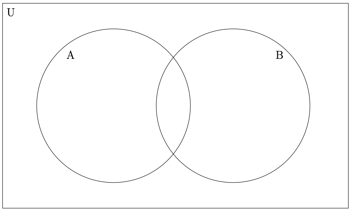
$clipboard_e02809234e0daa343b5b9da22cc50ccfa.png$

In a Venn diagram the universe of discourse is normally drawn as a rectangular region inside of which all the action occurs. Each set in a Venn diagram is depicted by drawing a simple closed curve – typically a circle, but not necessarily! For instance, if you want to draw a Venn diagram that shows all the possible intersections among four sets, you’ll find it’s impossible with (only) circles.

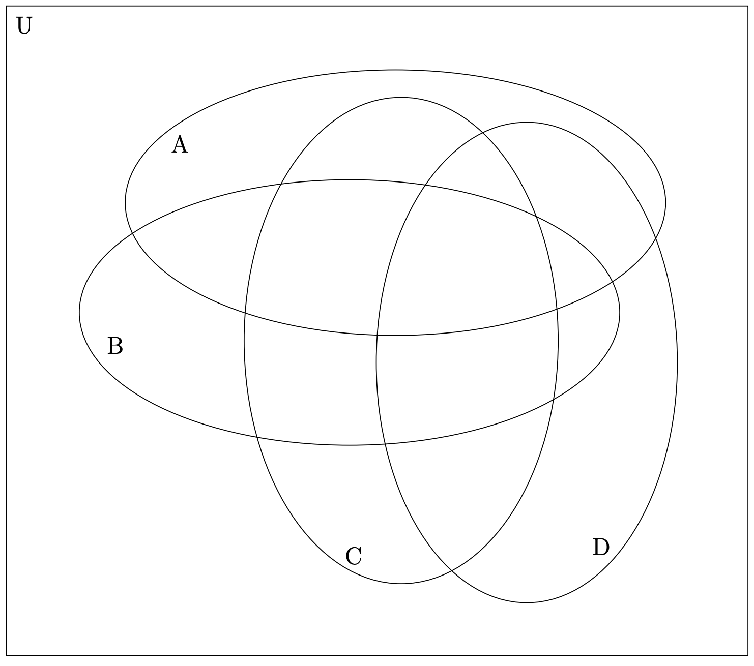
$clipboard_eeefb39678ca11a8da9865e5ebbb585c6.png$

Practice

Verify that the diagram above has regions representing all $16$ possible intersections of $4$ sets

There is a certain “zen” to Venn diagrams that must be internalized, but once you have done so they can be used to think very effectively about the relationships between sets. The main deal is that the points inside of one of the simple closed curves are not necessarily in the set – only some of the points inside a simple closed curve are in the set, and we don’t know precisely where they are! The various simple closed curves in a Venn diagram divide the universe up into a bunch of regions. It might be best to think of these regions as fenced-in areas in which the elements of a set mill about, much like domesticated animals in their pens. One of our main tools in working with Venn diagrams is to deduce that certain of these regions don’t contain any elements – we then mark that region with the emptyset symbol ($∅$).

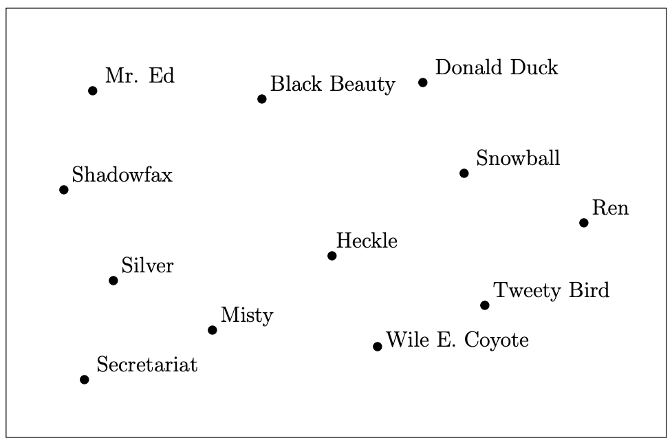
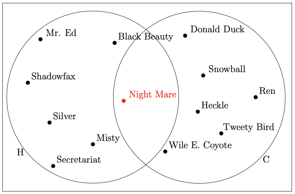
Here is a small example of a finite universe.

$clipboard_e37ce798828679e4d4ad7c3ab21ff51e4.png$

And here is the same universe with some Jordan curves used to encircle two subsets.

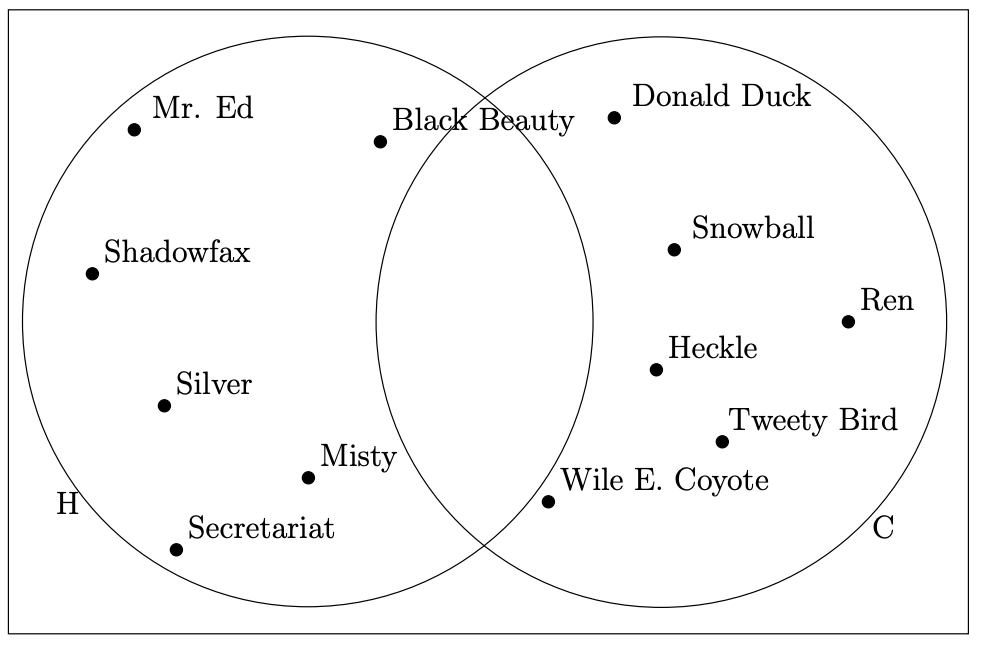
$clipboard_e34ccc081ad5e0c712e20a1778d3eba67.png$

This picture might lead us to think that the set of cartoon characters and the set of horses are disjoint, so we thought it would be nice to add one more element to our universe in order to dispel that notion.

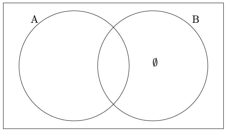
$clipboard_ef9d3b15b0507c3ee6ad11ad4513eca20.png$

Suppose we have two sets $A$ and $B$ and we’re interested in proving that $B ⊆ A$. The job is done if we can show that all of $B$’s elements are actually in the eye-shaped region that represents the intersection $A ∩ B$. It’s equivalent if we can show that the region marked with $∅$ in the following diagram is actually empty.

$clipboard_eb2e35bee0f931bec78e60f7aa01f5766.png$

Let’s put all this together. The inclusion $B ⊆ A$ corresponds to the logical sentence $M_B \implies M_A$. We know that implications are equivalent to OR statements, so $M_B \implies M_A \cong ¬M_B ∨ M_A$. The notion that the region we’ve indicated above is empty is written as $A ∩ B = ∅$, in logical terms this is $¬M_A ∧ M_B \cong c$. Finally, we apply DeMorgan’s law and a commutation to get $¬M_B ∨M_A \cong t$. You should take note of the convention that when you see a logical sentence just written on the page (as is the case with $M_B \implies M_A$ in the first sentence of this paragraph) what’s being asserted is that the sentence is universally true. Thus, writing $M_B \implies M_A$ is the same thing as writing $M_B =\implies M_A \cong t$.

One can use information that is known a priori when drawing a Venn diagram. For instance, if two sets are known to be disjoint, or if one is known to be contained in the other, we can draw Venn diagrams like the following

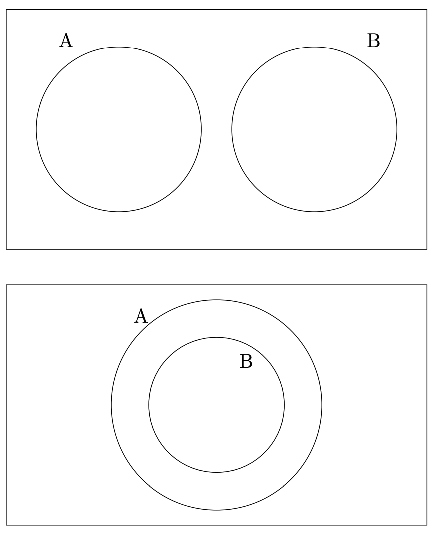
$clipboard_ecc9dc487558b01d4789f81b7a22e00a7.png$

However, both of these situations can also be dealt with by working with Venn diagrams in which the sets are in general position – which in this situation means that every possible intersection is shown – and then marking any empty regions with $∅$.

Practice

On a Venn diagram for two sets in general position, indicate the empty regions when

The sets are disjoint.
$A$ is contained in $B$.

$clipboard_e8750ab775566dbbff36c99019b30bdd3.png$

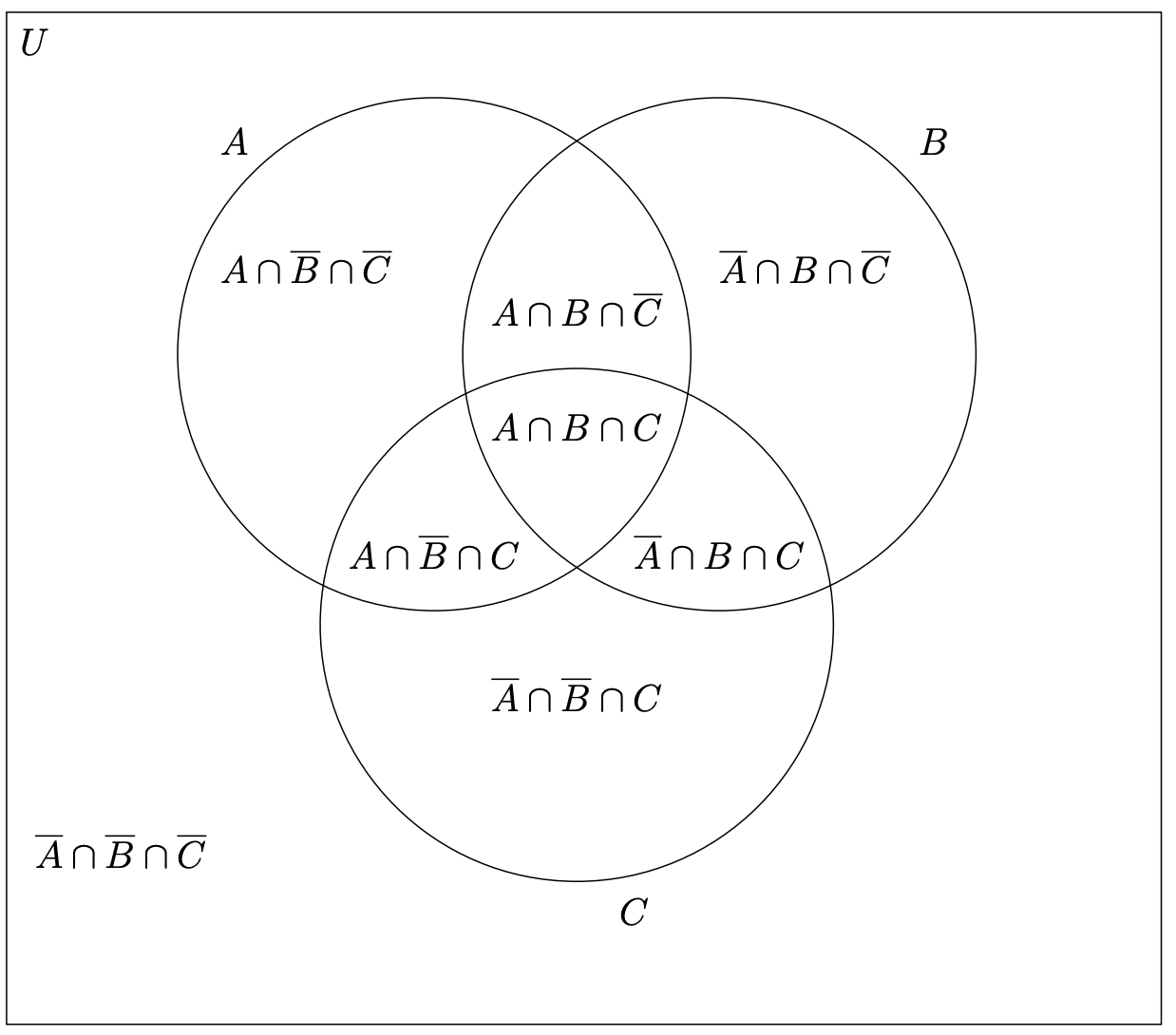
There is a connection, perhaps obvious, between the regions we see in a Venn diagram with sets in general position and the recognizers we studied in the section on digital logic circuits. In fact, both of these topics have to do with disjunctive normal form. In a Venn diagram with $k$ sets, we are seeing the universe of discourse broken up into the union of $2^k$ regions each of which corresponds to an intersection of either one of the sets or its complement. An arbitrary expression involving set-theoretic symbols and these $k$ sets is true in certain of these $2^k$ regions and false in the others. We have put the arbitrary expression in disjunctive normal form when we express it as a union of the intersections that describe those regions.

$clipboard_e674a9752c8281e2973568aa6323a0052.png$

Exercises:

Exercise $\PageIndex{1}$

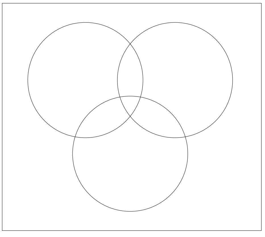
Let $A = \{1, 2, 4, 5\}$, $B = \{2, 3, 4, 6\}$, and $C = \{1, 2, 3, 4\}$. Place each of the elements $1, . . . , 6$ in the appropriate regions of a three-set Venn diagram.

$clipboard_e223033bd4e2e4fa59c4242613389237b.png$

Exercise $\PageIndex{2}$

Prove or disprove: $(A ∩ C ⊆ B ∩ C) \implies A ⊆ B$

Exercise $\PageIndex{3}$

Venn diagrams are usually made using simple closed curves with no further restrictions. Try creating Venn diagrams for $3$, $4$ and $5$ sets (in general position) using rectangular simple closed curves.

Exercise $\PageIndex{4}$

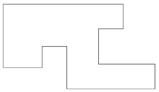
We call a curve rectilinear if it is made of line segments that meet at right angles. If you have ever played with an Etch-a-Sketch you’ll know what we mean by the term “rectilinear.” The following example of a rectilinear curve may also help to clarify this notion.

$clipboard_ee941773a502d6b3f0fbbc4ff77f5c1db.png$

Use rectilinear simple closed curves to create a Venn diagram for $5$ sets.

Exercise $\PageIndex{5}$

Argue as to why rectilinear curves will suffice to build any Venn diagram.

Exercise $\PageIndex{6}$

Find the disjunctive normal form of $A ∩ (B ∪ C)$.

Exercise $\PageIndex{7}$

Find the disjunctive normal form of $(A \triangle B) \triangle C$

Exercise $\PageIndex{8}$

The prototypes for the modus ponens and modus tollens argument forms are the following:

All men are mortal. All men are mortal.

Socrates is a man. and. Zeus is not mortal.

Therefore Socrates is mortal. Therefore Zeus is not a man.

Illustrate these arguments using Venn diagrams.

Exercise $\PageIndex{9}$

Use Venn diagrams to convince yourself of the validity of the following containment statement

$(A ∩ B) ∪ (C ∩ D) ⊆ (A ∪ C) ∩ (B ∪ D)$.

Now prove it!

Exercise $\PageIndex{10}$

Use Venn diagrams to show that the following set equivalence is false.

$(A ∪ B) ∩ (C ∪ D) = (A ∪ C) ∩ (B ∪ D)$

Search

Exercise \(\PageIndex{1}\)

Exercise \(\PageIndex{2}\)

Exercise \(\PageIndex{3}\)

Exercise \(\PageIndex{4}\)

Exercise \(\PageIndex{5}\)

Exercise \(\PageIndex{6}\)

Exercise \(\PageIndex{7}\)

Exercise \(\PageIndex{8}\)

Exercise \(\PageIndex{9}\)

Exercise \(\PageIndex{10}\)