3.2: Slope
- Page ID
- 19693

\( \newcommand{\vecs}[1]{\overset { \scriptstyle \rightharpoonup} {\mathbf{#1}} } \)
\( \newcommand{\vecd}[1]{\overset{-\!-\!\rightharpoonup}{\vphantom{a}\smash {#1}}} \)
\( \newcommand{\dsum}{\displaystyle\sum\limits} \)
\( \newcommand{\dint}{\displaystyle\int\limits} \)
\( \newcommand{\dlim}{\displaystyle\lim\limits} \)
\( \newcommand{\id}{\mathrm{id}}\) \( \newcommand{\Span}{\mathrm{span}}\)
( \newcommand{\kernel}{\mathrm{null}\,}\) \( \newcommand{\range}{\mathrm{range}\,}\)
\( \newcommand{\RealPart}{\mathrm{Re}}\) \( \newcommand{\ImaginaryPart}{\mathrm{Im}}\)
\( \newcommand{\Argument}{\mathrm{Arg}}\) \( \newcommand{\norm}[1]{\| #1 \|}\)
\( \newcommand{\inner}[2]{\langle #1, #2 \rangle}\)
\( \newcommand{\Span}{\mathrm{span}}\)
\( \newcommand{\id}{\mathrm{id}}\)
\( \newcommand{\Span}{\mathrm{span}}\)
\( \newcommand{\kernel}{\mathrm{null}\,}\)
\( \newcommand{\range}{\mathrm{range}\,}\)
\( \newcommand{\RealPart}{\mathrm{Re}}\)
\( \newcommand{\ImaginaryPart}{\mathrm{Im}}\)
\( \newcommand{\Argument}{\mathrm{Arg}}\)
\( \newcommand{\norm}[1]{\| #1 \|}\)
\( \newcommand{\inner}[2]{\langle #1, #2 \rangle}\)
\( \newcommand{\Span}{\mathrm{span}}\) \( \newcommand{\AA}{\unicode[.8,0]{x212B}}\)
\( \newcommand{\vectorA}[1]{\vec{#1}} % arrow\)
\( \newcommand{\vectorAt}[1]{\vec{\text{#1}}} % arrow\)
\( \newcommand{\vectorB}[1]{\overset { \scriptstyle \rightharpoonup} {\mathbf{#1}} } \)
\( \newcommand{\vectorC}[1]{\textbf{#1}} \)
\( \newcommand{\vectorD}[1]{\overrightarrow{#1}} \)
\( \newcommand{\vectorDt}[1]{\overrightarrow{\text{#1}}} \)
\( \newcommand{\vectE}[1]{\overset{-\!-\!\rightharpoonup}{\vphantom{a}\smash{\mathbf {#1}}}} \)
\( \newcommand{\vecs}[1]{\overset { \scriptstyle \rightharpoonup} {\mathbf{#1}} } \)
\(\newcommand{\longvect}{\overrightarrow}\)
\( \newcommand{\vecd}[1]{\overset{-\!-\!\rightharpoonup}{\vphantom{a}\smash {#1}}} \)
\(\newcommand{\avec}{\mathbf a}\) \(\newcommand{\bvec}{\mathbf b}\) \(\newcommand{\cvec}{\mathbf c}\) \(\newcommand{\dvec}{\mathbf d}\) \(\newcommand{\dtil}{\widetilde{\mathbf d}}\) \(\newcommand{\evec}{\mathbf e}\) \(\newcommand{\fvec}{\mathbf f}\) \(\newcommand{\nvec}{\mathbf n}\) \(\newcommand{\pvec}{\mathbf p}\) \(\newcommand{\qvec}{\mathbf q}\) \(\newcommand{\svec}{\mathbf s}\) \(\newcommand{\tvec}{\mathbf t}\) \(\newcommand{\uvec}{\mathbf u}\) \(\newcommand{\vvec}{\mathbf v}\) \(\newcommand{\wvec}{\mathbf w}\) \(\newcommand{\xvec}{\mathbf x}\) \(\newcommand{\yvec}{\mathbf y}\) \(\newcommand{\zvec}{\mathbf z}\) \(\newcommand{\rvec}{\mathbf r}\) \(\newcommand{\mvec}{\mathbf m}\) \(\newcommand{\zerovec}{\mathbf 0}\) \(\newcommand{\onevec}{\mathbf 1}\) \(\newcommand{\real}{\mathbb R}\) \(\newcommand{\twovec}[2]{\left[\begin{array}{r}#1 \\ #2 \end{array}\right]}\) \(\newcommand{\ctwovec}[2]{\left[\begin{array}{c}#1 \\ #2 \end{array}\right]}\) \(\newcommand{\threevec}[3]{\left[\begin{array}{r}#1 \\ #2 \\ #3 \end{array}\right]}\) \(\newcommand{\cthreevec}[3]{\left[\begin{array}{c}#1 \\ #2 \\ #3 \end{array}\right]}\) \(\newcommand{\fourvec}[4]{\left[\begin{array}{r}#1 \\ #2 \\ #3 \\ #4 \end{array}\right]}\) \(\newcommand{\cfourvec}[4]{\left[\begin{array}{c}#1 \\ #2 \\ #3 \\ #4 \end{array}\right]}\) \(\newcommand{\fivevec}[5]{\left[\begin{array}{r}#1 \\ #2 \\ #3 \\ #4 \\ #5 \\ \end{array}\right]}\) \(\newcommand{\cfivevec}[5]{\left[\begin{array}{c}#1 \\ #2 \\ #3 \\ #4 \\ #5 \\ \end{array}\right]}\) \(\newcommand{\mattwo}[4]{\left[\begin{array}{rr}#1 \amp #2 \\ #3 \amp #4 \\ \end{array}\right]}\) \(\newcommand{\laspan}[1]{\text{Span}\{#1\}}\) \(\newcommand{\bcal}{\cal B}\) \(\newcommand{\ccal}{\cal C}\) \(\newcommand{\scal}{\cal S}\) \(\newcommand{\wcal}{\cal W}\) \(\newcommand{\ecal}{\cal E}\) \(\newcommand{\coords}[2]{\left\{#1\right\}_{#2}}\) \(\newcommand{\gray}[1]{\color{gray}{#1}}\) \(\newcommand{\lgray}[1]{\color{lightgray}{#1}}\) \(\newcommand{\rank}{\operatorname{rank}}\) \(\newcommand{\row}{\text{Row}}\) \(\newcommand{\col}{\text{Col}}\) \(\renewcommand{\row}{\text{Row}}\) \(\newcommand{\nul}{\text{Nul}}\) \(\newcommand{\var}{\text{Var}}\) \(\newcommand{\corr}{\text{corr}}\) \(\newcommand{\len}[1]{\left|#1\right|}\) \(\newcommand{\bbar}{\overline{\bvec}}\) \(\newcommand{\bhat}{\widehat{\bvec}}\) \(\newcommand{\bperp}{\bvec^\perp}\) \(\newcommand{\xhat}{\widehat{\xvec}}\) \(\newcommand{\vhat}{\widehat{\vvec}}\) \(\newcommand{\uhat}{\widehat{\uvec}}\) \(\newcommand{\what}{\widehat{\wvec}}\) \(\newcommand{\Sighat}{\widehat{\Sigma}}\) \(\newcommand{\lt}{<}\) \(\newcommand{\gt}{>}\) \(\newcommand{\amp}{&}\) \(\definecolor{fillinmathshade}{gray}{0.9}\)In the previous section on Linear Models, we saw that if the dependent variable was changing at a constant rate with respect to the independent variable, then the graph was a line. If the rate was positive, then as we swept our eyes from left to right, the line rose upward, the dependent variable increasing with increasing changes in the independent variable. If the rate was negative, then the graph fell downward, the dependent variable decreasing with increasing changes in the independent variable. You may have also learned that higher rates led to steeper lines (lines that rose more quickly) and lower rates led to lines that were less steep.
In this section, we will connect the intuitive concept of rate developed in the previous section with a formal definition of the slope of a line. To start, let’s state up front what is meant by the slope of a line.
Slope is a number that tells us how quickly a line rises or falls.
If slope is a number that is directly connected to the “steepness” of a line, then we should have certain expectations.
- Lines with positive slope should slant uphill (as our eyes sweep from left to right).
- Lines with negative slope should slant downhill (as our eyes sweep from left to right).
- Because any horizontal line neither slants uphill nor downhill, we expect that it should have slope equal to zero.
- Lines with a larger positive slope should rise more quickly than lines with a smaller positive slope.
- If two lines have negative slope, then the line having the slope with larger absolute value should fall more quickly than the other line.
It remains to define how to compute the slope of a particular line. Whatever definition we choose, it should conform with the expectations outlined above. We also would like the definition of slope to conform with the concept of rate developed in the previous section. Thus, we make the following definition.
The slope of a line is the rate at which the dependent variable is changing with respect to the independent variable.
Note how the word “change” is used Definition. It is important to understand that the change in some quantity can be positive, negative, or zero. For example, if the temperature outside is \(40^{\circ} \mathrm{F}\) when I leave my home at 6 AM, and at noon the temperature is 65◦ F, then the change in temperature is a positive \(25^{\circ} \mathrm{F}\). On the other hand, if the temperature outside is \(65^{\circ} \mathrm{F}\) at noon, and the temperature is \(50^{\circ} \mathrm{F}\) when I return home in the evening, then the change in temperature is a negative 15 degrees Fahrenheit.
In calculating the change in a quantity, follow this rule.
Change in Quantity = Latter Measurement − Former Measurement.
Thus, if T represents the temperature and \(\Delta T\) represents the change in the temperature, then in our first case (taking the temperature in the morning then later at noon), the change in temperature is \[\Delta T=\text { Latter }-\text { Former }=65^{\circ} \mathrm{F}-40^{\circ} \mathrm{F}=25^{\circ} \mathrm{F} \nonumber \]
This positive result represents an increase in the temperature of \(25^{\circ} \mathrm{F}\).
In the second case (taking the temperature at noon then later in the evening), the change in temperature is
\[\begin{align*} \Delta T &= \text{Latter} - \text{Former} \\[4pt] &=50^{\circ} \mathrm{F}-65^{\circ} \mathrm{F} \\[4pt] &=-15^{\circ} \mathrm{F} \end{align*} \]
This negative result represents a decrease in the temperature of \(15^{\circ} \mathrm{F}\)
Readers should note that the direction of subtraction is extremely important. To detect the change in a quantity, always subtract the former (earlier) measurement from the latter (later) measurement.
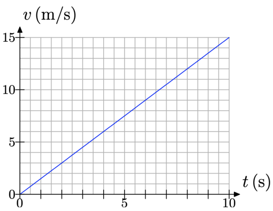
A ball is perched at rest at the top of a long ramp. It’s given a little tap and it begins to roll down the ramp. The speed v of the ball (in meters per second) is plotted versus the time t (in seconds) in Figure \(\PageIndex{1}\).
Determine the slope of the line.
Solution
We’ve defined the slope as the rate at which the dependent variable is changing with respect to the independent variable. In this case, the speed v of the ball “depends” upon the amount of time t that has elapsed. Consequently, v is the dependent variable and has been placed on the vertical axis.3 On the other hand, t is the independent variable and has been assigned the horizontal axis.
To determine the rate at which v is changing with respect to t (the slope of the line), we first select two points P(2, 3) and Q(8, 12) on the line, as shown in Figure \(\PageIndex{2}\). As we sweep our eyes from left to right (a convention we will always follow when dealing with slope), the point P occurs before the point Q. Hence, we consider P the “former” measurement and point Q the “latter” measurement.
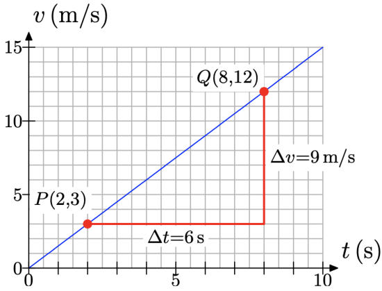
At point P, the time is t = 2 seconds, then at point Q the time is t = 8 seconds. The change in t is found by subtracting the former measurement from the latter measurement.
\[\Delta t=8 s-2 s=6 s \nonumber \]
At point P, the speed is v = 3 meters per second, then at point Q the speed is v = 12 meters per second. Hence, the change in v is
\[\Delta v=12 \mathrm{m} / \mathrm{s}-3 \mathrm{m} / \mathrm{s}=9 \mathrm{m} / \mathrm{s} \nonumber \]
Finally, the slope of the line is defined as the rate at which the dependent variable v is changing with respect to the independent variable t. That is,
\[\text { Slope }=\frac{\Delta v}{\Delta t}=\frac{9 \mathrm{m} / \mathrm{s}}{6 \mathrm{s}}=\frac{3 \mathrm{m} / \mathrm{s}}{\mathrm{s}} \nonumber \]
Scientists prefer to write this as 1.5 \(\mathrm{m} / \mathrm{s}^{2}\), but this might not be as intuitive as writing 1.5 (m/s)/s, which indicates that the speed is increasing at a rate of 1.5 m/s every second. This makes good sense as a ball rolling down a ramp will pick up speed with the passage of time. The slope provides an exact numerical description of how the speed increases with respect to time.
Note that our definition of the slope of the line satisfies one of our goals: the slope is precisely the same as the notion of rate described in the previous section. Indeed, note the right triangle we’ve drawn in Figure \(\PageIndex{2}\). The bottom edge of the triangle is 12 boxes long, but every 2 boxes represents one second, so this displacement in the time t direction is 6 seconds. The vertical side of the right triangle is 9 boxes in height where each box represents 1 meter per second. Consequently, this vertical edge of the right triangle represents a positive displacement of 9 meters per second. Thus, every 6 seconds, there is an increase in speed of 9 meters per second. Hence, the ball is picking up speed at the rate of 9 meters per second every 6 seconds, or equivalently, 1.5 meters per second every second.
In Figure \(\PageIndex{2}\), the rate at which the speed is increasing with respect to time is equivalent to the slope of the line.
Suppose that we had labeled our points \(P\left(t_{\text { initial }}, v_{\text { initial }}\right)\) and \(Q\left(t_{\text { final }}, v_{\text { final }}\right)\) as shown in Figure \(\PageIndex{3}\).
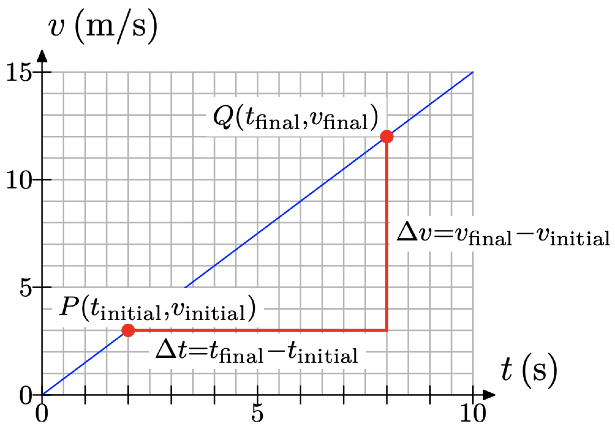
Now the change in speed v would be
\[\Delta v=v_{\text { final }}-v_{\text { initial }} \nonumber \]
and the change in time t would be
\[\Delta t=t_{\text { final }}-t_{\text { initial }} \nonumber \]
Therefore, the slope of the line would be computed with the following formula.
\[\text { Slope }=\frac{\Delta v}{\Delta t}=\frac{v_{\text { final }}-v_{\text { initial }}}{t_{\text { final }}-t_{\text { initial }}}\nonumber \]
With \(P\left(t_{\text { initial }}, v_{\text { initial }}\right)=(2 \mathrm{s}, 3 \mathrm{m} / \mathrm{s})\) and \(Q\left(t_{\text { final }}, v_{\text { final }}\right)=(8 \mathrm{s}, 12 \mathrm{m} / \mathrm{s}),\) this becomes
\[\text { Slope }=\frac{12 \mathrm{m} / \mathrm{s}-3 \mathrm{m} / \mathrm{s}}{8 \mathrm{s}-2 \mathrm{s}}=\frac{9 \mathrm{m} / \mathrm{s}}{6 \mathrm{s}}=1.5 \mathrm{m} / \mathrm{s}^{2} \nonumber \]
The Slope Formula
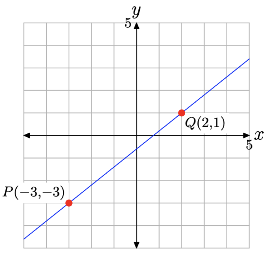
The last calculation in Example \(\PageIndex{1}\) allows us to discuss the slope of a line as a purely mathematical concept, one that is not rooted in a supporting application as in Example \(\PageIndex{1}\). Take, for example, the line shown in Figure \(\PageIndex{4}\) that passes through the points \(P(−3, −3)\) and \(Q(2, 1)\).
In this example, the dependent variable is y and the independent variable is x, so the slope of the line is \(\Delta y\) (the change in y) divided by \(\Delta x\) (the change in x).
\[\text { Slope }=\frac{\Delta y}{\Delta x} \nonumber \]
Sweeping our eyes from left to right, the point P comes first, followed by the point Q. Keeping “latter minus former” in mind, the change in y is computed by subtracting the y-value of point P from the y-value of point Q. That is,
\[\Delta y=1-(-3)=4 \nonumber \]
Similarly, the change in x is computed by subtracting the x-value of point P from the x-value of point Q. That is,
\[\Delta x=2-(-3)=5 \nonumber \]
Thus, the slope of the line is
\[\text { Slope }=\frac{\Delta y}{\Delta x}=\frac{4}{5} \nonumber \]
Alternatively, we can use the points P and Q as vertices of a right triangle with sides parallel to the axes (shown in Figure \(\PageIndex{5}\)(a)). The horizontal edge of the right triangle is 5 boxes (each representing 1 unit), so the displacement in x is 5 units. The vertical edge is 4 boxes (each representing 1 unit), so the displacement in y is 4 units. Hence, each time x is increased by 5 units, y experiences an increase of 4 units. Therefore, the slope of the line is again 4/5.
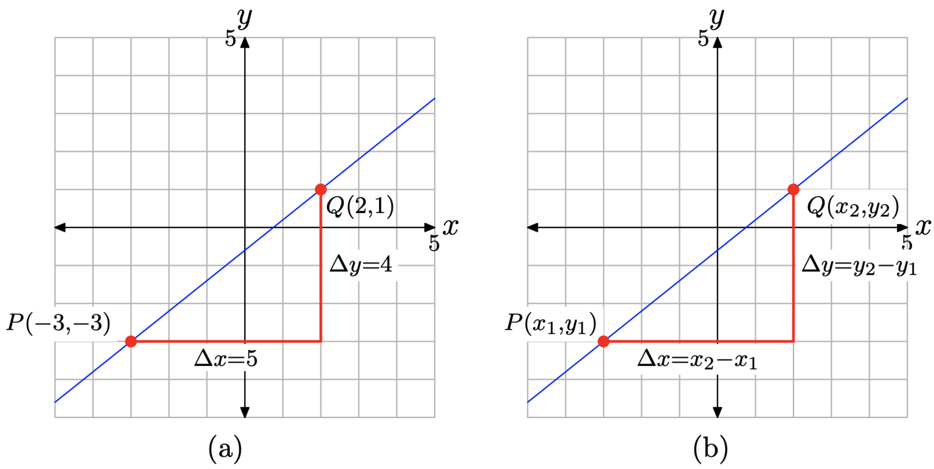
Suppose that we had labeled our points \(P\left(x_{1}, y_{1}\right)\) and \(Q\left(x_{2}, y_{2}\right)\) as shown in Figure \(\PageIndex{5}\)(b). Now the change in y would be
\[\Delta y=y_{2}-y_{1} \nonumber \]
and the change in x would be
\[\Delta x=x_{2}-x_{1} \nonumber \]
Therefore, the slope of the line would be computed with the following formula.
\[\text { Slope }=\frac{\Delta y}{\Delta x}=\frac{y_{2}-y_{1}}{x_{2}-x_{1}} \nonumber \]
With \(P\left(x_{1}, y_{1}\right)=(-3,-3)\) and \(Q\left(x_{2}, y_{2}\right)=(2,1),\) this becomes
\[\text { Slope }=\frac{1-(-3)}{2-(-3)}=\frac{4}{5} \nonumber \]
The slope formula is worth summarizing in a definition.
The slope of the line that passes through the points \(P\left(x_{1}, y_{1}\right)\) and \(Q\left(x_{2}, y_{2}\right)\) is given by the formula
\[\text {Slope }=\frac{\Delta y}{\Delta x}=\frac{y_{2}-y_{1}}{x_{2}-x_{1}} \nonumber \]
Let’s look at some more examples.
Find the slope of the line passing through the points P(−3, −2) and Q(3, 1).
Solution
We can use the slope formula in Definition 5 to determine the slope. With \(\left(x_{1}, y_{1}\right)=P(-3,-2)\) and \(\left(x_{2}, y_{2}\right)=Q(3,1)\),
\[\text { Slope }=\frac{\Delta y}{\Delta x}=\frac{y_{2}-y_{1}}{x_{2}-x_{1}}=\frac{1-(-2)}{3-(-3)}=\frac{3}{6}=\frac{1}{2} \nonumber \]
Readers will sometimes ask, “Which point should be \(\left(x_{1}, y_{1}\right)\) and which should be \(\left(x_{2}, y_{2}\right)\)?” The short answer is, “It doesn’t matter!” Suppose instead, that we let \(\left(x_{1}, y_{1}\right)=Q(3,1)\) and \(\left(x_{2}, y_{2}\right)=P(-3,-2)\). Then,
\[\text { Slope }=\frac{\Delta y}{\Delta x}=\frac{y_{2}-y_{1}}{x_{2}-x_{1}}=\frac{-2-1}{-3-3}=\frac{-3}{-6}=\frac{1}{2} \nonumber \]
Because the change in any quantity is found by subtracting the earlier measurement from the later measurement, we will continue to stress the first order. However, if we reverse the points as we did in our second calculation, both numerator and denominator reverse sign with this interchange, so we get the same answer.
Of course, we can also determine the slope by plotting P(−3, −2) and Q(3, 1) and the line that passes through P and Q, as we’ve done in Figure \(\PageIndex{6}\).
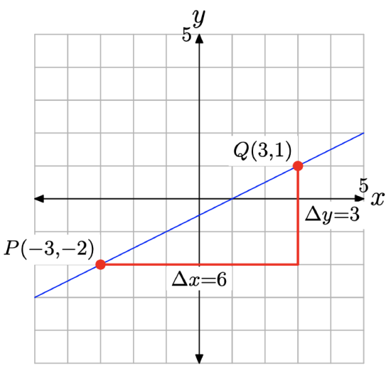
Starting at the point P, to get to the point Q, we move 6 boxes to the right, then 3 boxes up, as shown in Figure \(\PageIndex{6}\). Hence, the slope of the line is
\[\text { Slope }=\frac{\Delta y}{\Delta x}=\frac{3}{6}=\frac{1}{2} \nonumber \]
Note that two of our expectations regarding the slope of a line are met with this example.
- The line through P(−3, −2) and Q(3, 1) in Figure \(\PageIndex{6}\) has slope 1/2. This is a positive number and the line slants uphill (as expected) as we sweep our eyes from left to right.
- The slope in this example is 1/2, which is less than the slope of the line in Figure \(\PageIndex{5}\)(a), which was 4/5. Note that the line in Figure \(\PageIndex{6}\) is less steep than the line in Figure \(\PageIndex{5}\)(a), which was another of our earlier expectations regarding the slope of a line.
Find the slope of the line passing through the points P(−4, 4) and Q(4, −2).
Solution
We can use the slope formula in Definition 5 to determine the slope. With \(\left(x_{1}, y_{1}\right)=P(-4,4)\) and \(\left(x_{2}, y_{2}\right)=Q(4,-2)\),
\[\text { Slope }=\frac{\Delta y}{\Delta x}=\frac{y_{2}-y_{1}}{x_{2}-x_{1}}=\frac{-2-4}{4-(-4)}=\frac{-6}{8}=-\frac{3}{4} \nonumber \]
We can also get the slope of the line from the graph in Figure \(\PageIndex{7}\). Starting at the point P(−4, 4), move 8 units to the right, then 6 units downward, as shown in Figure \(\PageIndex{7}\).
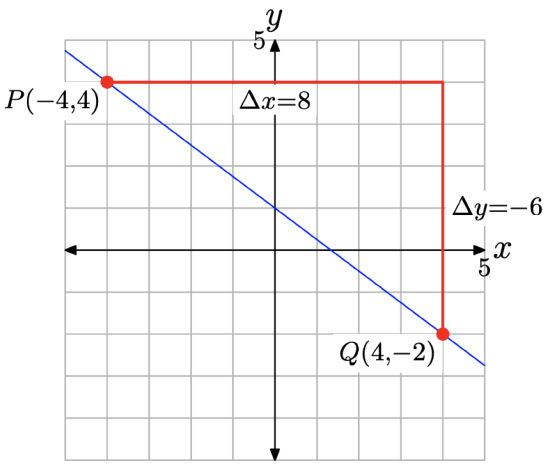
Thus, the slope of the line is
\[\text { Slope }=\frac{\Delta y}{\Delta x}=\frac{-6}{8}=-\frac{3}{4} \nonumber \]
Again, one of our earlier expectations regarding the slope of a line is met in this example. The slope is −3/4, which is a negative number, and the line in Figure \(\PageIndex{7}\) slants downhill (as we sweep our eyes from left to right).
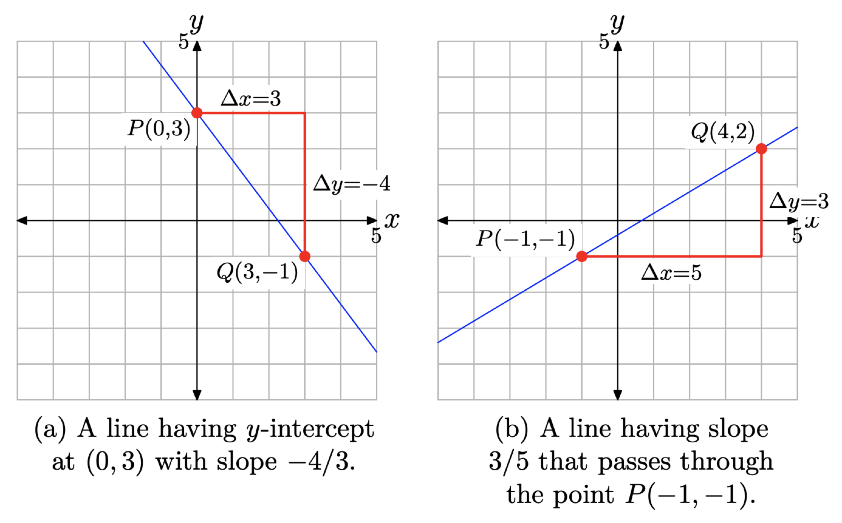
Draw a line that intercepts the y-axis at (0, 3) so that the line has slope −4/3. Draw a second line that passes through the point P(−1, −1) with slope 3/5.
Solution
The slope of the first line is −4/3. This means that our line must slant downhill (as we sweep our eyes from left to right). The slope is the change in y over the change in x. Therefore, every time x increases by 3 units, y must decrease by 4 units. Plot the point P(0, 3), as shown in Figure \(\PageIndex{8}\)(a). Then, starting at P, move 3 units to the right, followed by 4 units downward to the point Q(3, −1), as shown in Figure \(\PageIndex{8}\)(a). Draw the required line, which must pass through the points P and Q.
To draw the second line, first plot the point P(−1, −1), as shown in Figure \(\PageIndex{8}\)(b). Starting at the point P, move 5 units to the right, then upward 3 units to the point Q(4, 2), as shown in Figure \(\PageIndex{8}\)(b). Draw the required line passing through the points P and Q.
Parallel Lines
Because slope controls the “steepness” of a line, it is a simple matter to see that parallel lines must have the same slope.
Let \(\boldsymbol{L}_{1}\) be a line having slope \(m_{1}\). Let \(\boldsymbol{L}_{2}\) be a line having slope \(m_{2}\). If \(\boldsymbol{L}_{1}\) and \(\boldsymbol{L}_{2}\) are parallel, then
\[m_{1}=m_{2} \nonumber \]
That is, any two parallel lines have the same slope.
What is the slope of any horizontal line? What is the slope of any vertical line?
Solution
One would expect that our definition would verify that the slope of any horizontal line is zero. Select, for example, the horizontal line shown in Figure 9(a). Select the points (−3, 3) and (3, 3) on this line.
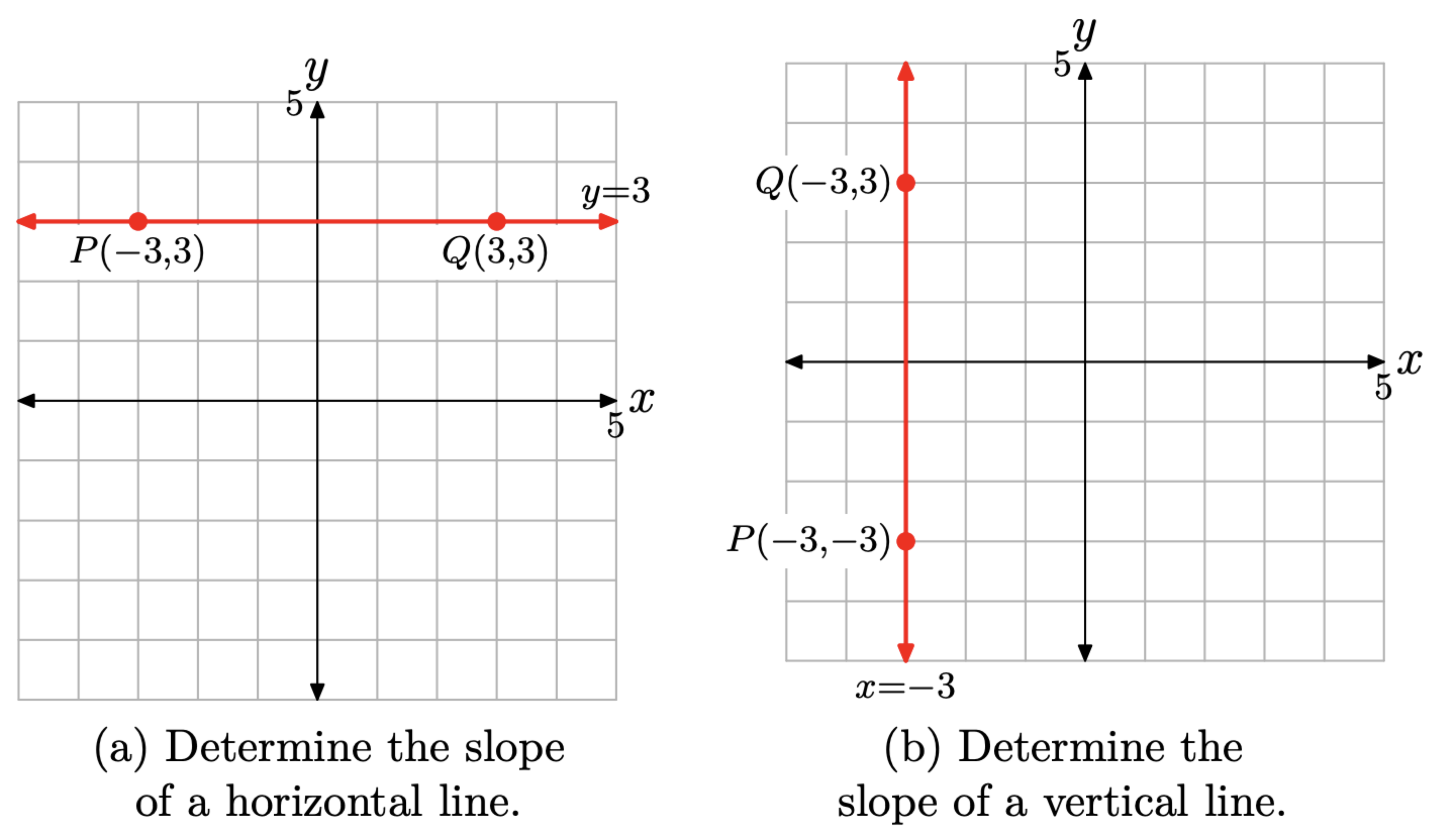
With \(\left(x_{1}, y_{1}\right)=(-3,3)\) and \(\left(x_{2}, y_{2}\right)=(3,3)\)
\[\text { Slope }=\frac{\Delta y}{\Delta x}=\frac{y_{2}-y_{1}}{x_{2}-x_{1}}=\frac{3-3}{3-(-3)}=\frac{0}{6}=0 \nonumber \]
Thus, the horizontal line in Figure \(\PageIndex{9}\)(a) has slope equal to zero, exactly as expected. Further, all horizontal lines are parallel to this horizontal line and have the same slope. Therefore, all horizontal lines have slope zero.
We would surmise that the vertical line in Figure \(\PageIndex{9}\)(b) has undefined slope (we’ll explore this more fully in the exercises). In Figure \(\PageIndex{9}\)(b), we’ve selected the points P(−3, −3) and Q(−3, 3) on the vertical line. With \(\left(x_{1}, y_{1}\right)=P(-3,-3)\) and \(\left(x_{2}, y_{2}\right)=Q(-3,-3)\), \[\text { Slope }=\frac{\Delta y}{\Delta x}=\frac{y_{2}-y_{1}}{x_{2}-x_{1}}=\frac{3-(-3)}{-3-(-3)}=\frac{6}{0}, \text { which is undefined. } \nonumber \]
The slope of the vertical line in Figure \(\PageIndex{9}\)(b) is undefined because division by zero is meaningless. Further, all vertical lines are parallel to this vertical line and have undefined slope.
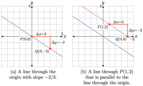
Draw a line through the point P(1, 2) that is parallel to the line passing through the origin with slope −2/3.
Solution
We will first draw a line through the origin with slope −2/3. Plot the point P(0, 0), then move 3 units to the right and 2 units downward to the point Q(3, −2), as shown in Figure \(\PageIndex{10}\)(a). Draw a line through the points P and Q as shown in Figure \(\PageIndex{10}\)(a).
Next, plot the point P(1, 2) as shown in Figure \(\PageIndex{10}\)(b). To draw a line through this point that is parallel to the line through the origin, this second line must have the same slope as the first line. Therefore, start at the point P(1, 2), as shown in Figure \(\PageIndex{10}\)(b), then move 3 units to the right and 2 units downward to the point Q(4, 0). Draw a line through the points P and Q as shown in Figure \(\PageIndex{10}\)(b). Note that this second line is parallel to the first.
Perpendicular Lines
The relationship between the slopes of two perpendicular lines is not as straightforward as the relation between the slopes of two parallel lines. Let’s begin by stating the pertinent property.
Let \(L_{1}\) be a line having slope \(m_{1}\). Let \(L_{2}\) be a line having slope \(m_{2}\). If \(L_{1}\) and \(L_{2}\) are perpendicular, then
\[m_{1} m_{2}=-1 \nonumber \]
That is, the product of the slopes of two perpendicular lines is −1.
We can solve equation (14) for \(m_{1}\) in terms of \(m_{2}\).
\[m_{1}=-\frac{1}{m_{2}} \nonumber \]
Equation (15) tells us that the slope of the first line is the negative reciprocal of the slope of the second line.
For example, suppose that \(L_{1}\) and \(L_{2}\) are perpendicular lines with slopes \(m_{1}\) and \(m_{2}\), respectively
- If \(m_{2}=2,\) then \(m_{1}=-\frac{1}{2}\)
- If \(m_{2}=\frac{3}{5},\) then \(m_{1}=-\frac{5}{3}\)
- If \(m_{2}=-\frac{2}{3},\) then \(m_{1}=\frac{3}{2}\)
Note that in each bulleted item, the product of the slopes is −1.
We won’t provide a proof of equation (15), but we will provide some motivating evidence in the form of a graph.
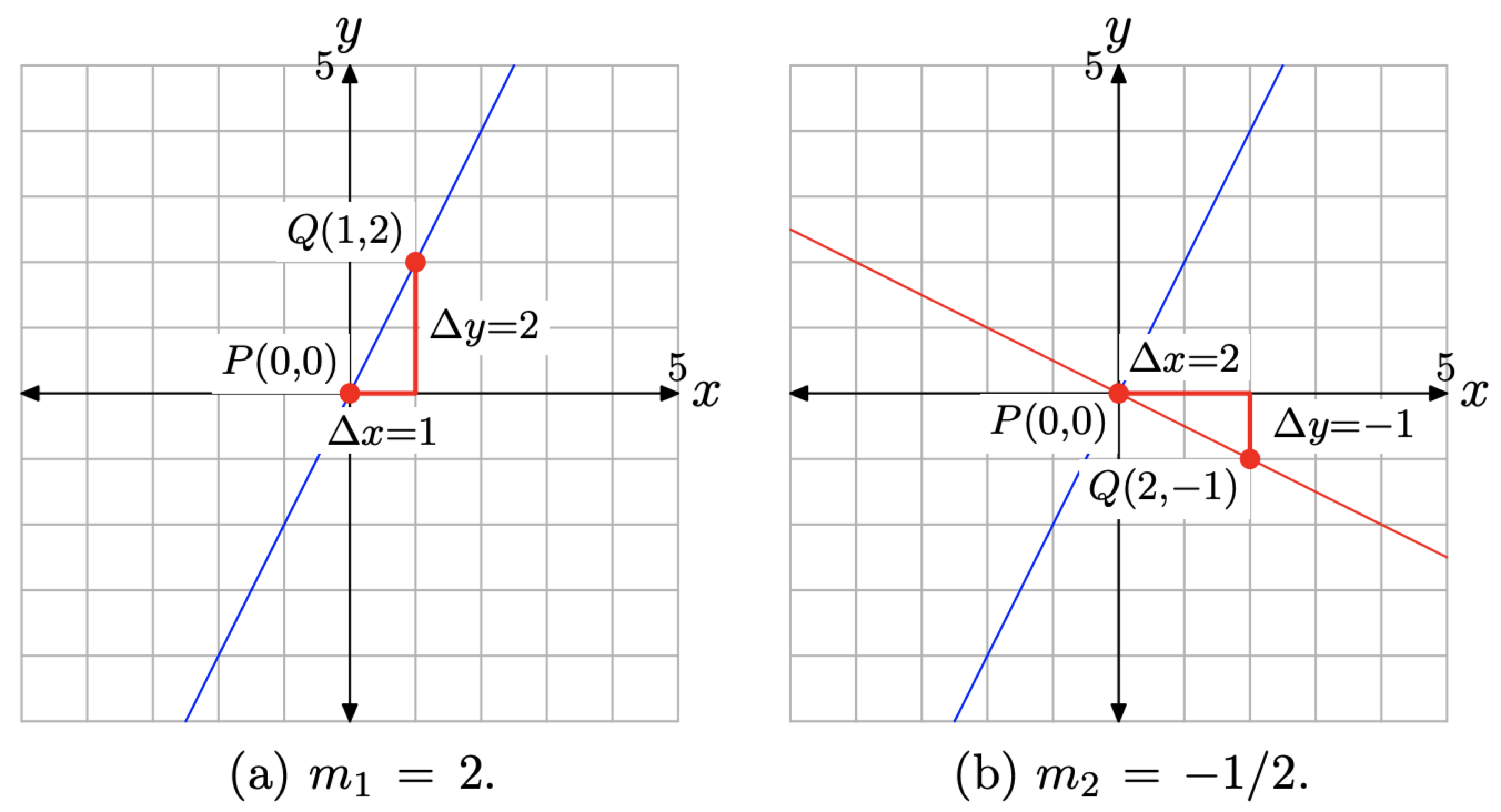
Sketch the graphs of the lines passing through the origin having slopes 2 and −1/2.
Solution
In Figure \(\PageIndex{11}\)(a), we’ve plotted the point P(0, 0) at the origin, then moved 1 unit to the right and 2 units upward to the point Q(1, 2). The resulting line passes through the origin and has slope \(m_{1}=2\) (alternatively, \(m_{1}=2 / 1\)).
In Figure \(\PageIndex{11}\)(b), we’ve again plotted the point P(0, 0) at the origin, then moved 2 units to the right and 1 unit downward to the point Q(2, −1). The resulting line passes through the origin and has slope \(m_{2}=-1 / 2\).
There are two important points that need to be made about the lines in Figure \(\PageIndex{11}\)(b).
The two lines in Figure \(\PageIndex{11}\)(b) are perpendicular. They meet and form a right angle of \(90^{\circ}\). If you have a protractor available, you might want to measure the angle between the two lines and note that the measure of the angle is \(90^{\circ}\).
The product of the two slopes is
\[m_{1} m_{2}=2 \cdot\left(-\frac{1}{2}\right)=-1 \nonumber \]