3.1: Linear Models
- Page ID
- 19692
\( \newcommand{\vecs}[1]{\overset { \scriptstyle \rightharpoonup} {\mathbf{#1}} } \)
\( \newcommand{\vecd}[1]{\overset{-\!-\!\rightharpoonup}{\vphantom{a}\smash {#1}}} \)
\( \newcommand{\dsum}{\displaystyle\sum\limits} \)
\( \newcommand{\dint}{\displaystyle\int\limits} \)
\( \newcommand{\dlim}{\displaystyle\lim\limits} \)
\( \newcommand{\id}{\mathrm{id}}\) \( \newcommand{\Span}{\mathrm{span}}\)
( \newcommand{\kernel}{\mathrm{null}\,}\) \( \newcommand{\range}{\mathrm{range}\,}\)
\( \newcommand{\RealPart}{\mathrm{Re}}\) \( \newcommand{\ImaginaryPart}{\mathrm{Im}}\)
\( \newcommand{\Argument}{\mathrm{Arg}}\) \( \newcommand{\norm}[1]{\| #1 \|}\)
\( \newcommand{\inner}[2]{\langle #1, #2 \rangle}\)
\( \newcommand{\Span}{\mathrm{span}}\)
\( \newcommand{\id}{\mathrm{id}}\)
\( \newcommand{\Span}{\mathrm{span}}\)
\( \newcommand{\kernel}{\mathrm{null}\,}\)
\( \newcommand{\range}{\mathrm{range}\,}\)
\( \newcommand{\RealPart}{\mathrm{Re}}\)
\( \newcommand{\ImaginaryPart}{\mathrm{Im}}\)
\( \newcommand{\Argument}{\mathrm{Arg}}\)
\( \newcommand{\norm}[1]{\| #1 \|}\)
\( \newcommand{\inner}[2]{\langle #1, #2 \rangle}\)
\( \newcommand{\Span}{\mathrm{span}}\) \( \newcommand{\AA}{\unicode[.8,0]{x212B}}\)
\( \newcommand{\vectorA}[1]{\vec{#1}} % arrow\)
\( \newcommand{\vectorAt}[1]{\vec{\text{#1}}} % arrow\)
\( \newcommand{\vectorB}[1]{\overset { \scriptstyle \rightharpoonup} {\mathbf{#1}} } \)
\( \newcommand{\vectorC}[1]{\textbf{#1}} \)
\( \newcommand{\vectorD}[1]{\overrightarrow{#1}} \)
\( \newcommand{\vectorDt}[1]{\overrightarrow{\text{#1}}} \)
\( \newcommand{\vectE}[1]{\overset{-\!-\!\rightharpoonup}{\vphantom{a}\smash{\mathbf {#1}}}} \)
\( \newcommand{\vecs}[1]{\overset { \scriptstyle \rightharpoonup} {\mathbf{#1}} } \)
\(\newcommand{\longvect}{\overrightarrow}\)
\( \newcommand{\vecd}[1]{\overset{-\!-\!\rightharpoonup}{\vphantom{a}\smash {#1}}} \)
\(\newcommand{\avec}{\mathbf a}\) \(\newcommand{\bvec}{\mathbf b}\) \(\newcommand{\cvec}{\mathbf c}\) \(\newcommand{\dvec}{\mathbf d}\) \(\newcommand{\dtil}{\widetilde{\mathbf d}}\) \(\newcommand{\evec}{\mathbf e}\) \(\newcommand{\fvec}{\mathbf f}\) \(\newcommand{\nvec}{\mathbf n}\) \(\newcommand{\pvec}{\mathbf p}\) \(\newcommand{\qvec}{\mathbf q}\) \(\newcommand{\svec}{\mathbf s}\) \(\newcommand{\tvec}{\mathbf t}\) \(\newcommand{\uvec}{\mathbf u}\) \(\newcommand{\vvec}{\mathbf v}\) \(\newcommand{\wvec}{\mathbf w}\) \(\newcommand{\xvec}{\mathbf x}\) \(\newcommand{\yvec}{\mathbf y}\) \(\newcommand{\zvec}{\mathbf z}\) \(\newcommand{\rvec}{\mathbf r}\) \(\newcommand{\mvec}{\mathbf m}\) \(\newcommand{\zerovec}{\mathbf 0}\) \(\newcommand{\onevec}{\mathbf 1}\) \(\newcommand{\real}{\mathbb R}\) \(\newcommand{\twovec}[2]{\left[\begin{array}{r}#1 \\ #2 \end{array}\right]}\) \(\newcommand{\ctwovec}[2]{\left[\begin{array}{c}#1 \\ #2 \end{array}\right]}\) \(\newcommand{\threevec}[3]{\left[\begin{array}{r}#1 \\ #2 \\ #3 \end{array}\right]}\) \(\newcommand{\cthreevec}[3]{\left[\begin{array}{c}#1 \\ #2 \\ #3 \end{array}\right]}\) \(\newcommand{\fourvec}[4]{\left[\begin{array}{r}#1 \\ #2 \\ #3 \\ #4 \end{array}\right]}\) \(\newcommand{\cfourvec}[4]{\left[\begin{array}{c}#1 \\ #2 \\ #3 \\ #4 \end{array}\right]}\) \(\newcommand{\fivevec}[5]{\left[\begin{array}{r}#1 \\ #2 \\ #3 \\ #4 \\ #5 \\ \end{array}\right]}\) \(\newcommand{\cfivevec}[5]{\left[\begin{array}{c}#1 \\ #2 \\ #3 \\ #4 \\ #5 \\ \end{array}\right]}\) \(\newcommand{\mattwo}[4]{\left[\begin{array}{rr}#1 \amp #2 \\ #3 \amp #4 \\ \end{array}\right]}\) \(\newcommand{\laspan}[1]{\text{Span}\{#1\}}\) \(\newcommand{\bcal}{\cal B}\) \(\newcommand{\ccal}{\cal C}\) \(\newcommand{\scal}{\cal S}\) \(\newcommand{\wcal}{\cal W}\) \(\newcommand{\ecal}{\cal E}\) \(\newcommand{\coords}[2]{\left\{#1\right\}_{#2}}\) \(\newcommand{\gray}[1]{\color{gray}{#1}}\) \(\newcommand{\lgray}[1]{\color{lightgray}{#1}}\) \(\newcommand{\rank}{\operatorname{rank}}\) \(\newcommand{\row}{\text{Row}}\) \(\newcommand{\col}{\text{Col}}\) \(\renewcommand{\row}{\text{Row}}\) \(\newcommand{\nul}{\text{Nul}}\) \(\newcommand{\var}{\text{Var}}\) \(\newcommand{\corr}{\text{corr}}\) \(\newcommand{\len}[1]{\left|#1\right|}\) \(\newcommand{\bbar}{\overline{\bvec}}\) \(\newcommand{\bhat}{\widehat{\bvec}}\) \(\newcommand{\bperp}{\bvec^\perp}\) \(\newcommand{\xhat}{\widehat{\xvec}}\) \(\newcommand{\vhat}{\widehat{\vvec}}\) \(\newcommand{\uhat}{\widehat{\uvec}}\) \(\newcommand{\what}{\widehat{\wvec}}\) \(\newcommand{\Sighat}{\widehat{\Sigma}}\) \(\newcommand{\lt}{<}\) \(\newcommand{\gt}{>}\) \(\newcommand{\amp}{&}\) \(\definecolor{fillinmathshade}{gray}{0.9}\)Sebastian waves good-bye to his brother, who is talking to a group of his friends approximately 20 feet away. Sebastian then begins to walk away from his brother at a constant rate of 4 feet per second. Let’s model the distance separating the two brothers as a function of time.
Our first approach will be graphical. We will let the variable d represent the distance (in feet) between the brothers and the variable t represent the amount of time (in seconds) that has passed since Sebastian waved good-bye to his brother. Because the distance separating the brothers depends on the amount of time that has passed, we will say that the distance d is the dependent variable and the time t is the independent variable.
It is somewhat traditional in the modeling process to place the independent variable on the horizontal axis and the dependent variable on the vertical axis. This is not a hard and fast rule, more a matter of personal taste, but we will follow this rule in our example nonetheless. Thus, we will place distance on the vertical axis and time on the horizontal axis, as shown in Figure \(\PageIndex{1}\). Notice that we’ve labeled each axis with its variable representation and included the units, an important practice.
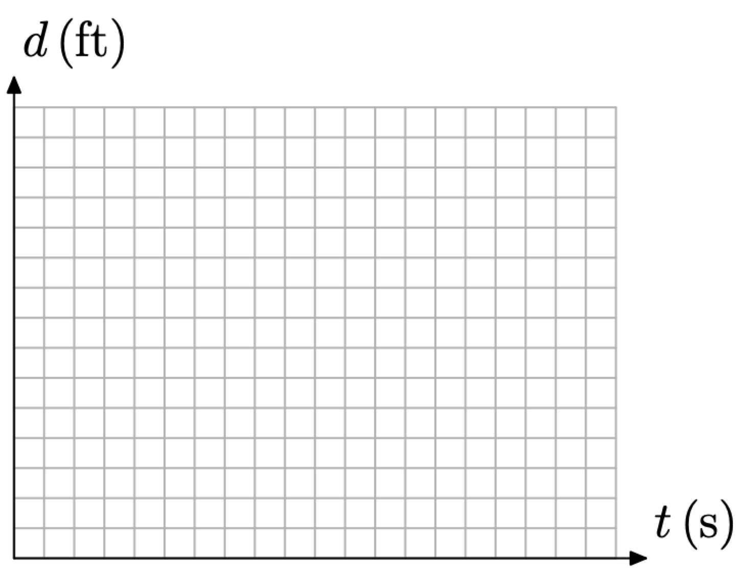
Figure \(\PageIndex{1}\). Distance depends upon time.
The label on the horizontal axis, t(s), might look like function notation to some readers. This is not the case. Rather, the variable t represents time, and the (s) in parentheses that follows represents seconds, a standard abbreviation in physics. Similar comments are in order for the label d (ft). The variable d represents distance, and the (ft) in parentheses that follows represent feet, another standard abbreviation in physics.
There are a number of different ways that you can label the axes of your graph with units appropriate for the problem at hand. For example, consider the technique presented in Figure \(\PageIndex{2}\), where the labels are placed to the left of the vertical axis and underneath the horizontal axis. Another difference is the fact that the unit abbreviations in Figure 1 are spelled out in their entirety in Figure \(\PageIndex{2}\).
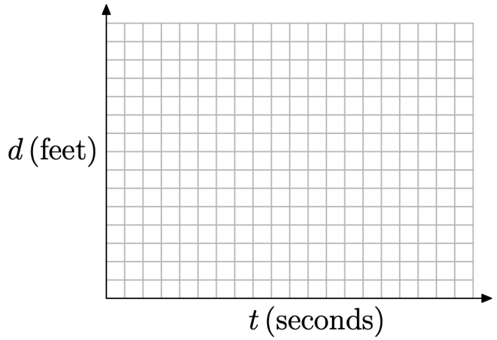
Figure \(\PageIndex{2}\). Distance depends upon time.
Some instructors prefer that you rotate the distance label on the vertical axis ninety degrees, so that it appears sideways. Others prefer that you label the ends of each axis with the variable, as we have done in Figure \(\PageIndex{1}\), but spell out the units in their entirety alongside each axis as we’ve done in Figure \(\PageIndex{2}\). The list of preferences goes on and on.
It is important to have a conversation with your instructor in order to determine what your instructor’s expectations are when it comes to labeling the axes and indicating the units on your graphs.
We prefer to label the axes as shown in Figure \(\PageIndex{1}\), and we will try to be consistent to this standard throughout the remainder of the text, though we might stray to alternate forms of labeling from time to time
We must now scale each axis appropriately, a task that is harder than it first seems. A poor choice of scale can make the task ahead more difficult than it needs to be. We will choose a scale for each axis with the following thoughts in mind.
Here is some good advice to follow when scaling the dependent and independent axes.
- We want to avoid postage-stamp-sized graphs. A large graph is easier to interpret than one that is cramped in a small corner of our graph paper.
- It is not necessary to have the same scale on each axis, but once a scale is chosen, you must remain consistent.
- We want to choose a scale that correlates easily with the given rate.
Sebastian is walking away from his brother at a constant rate of 4 feet per second. Let’s let each box on the vertical axis represent 4 feet and every two boxes on the horizontal axis represent 1 second, as shown in Figure \(\PageIndex{3}\).
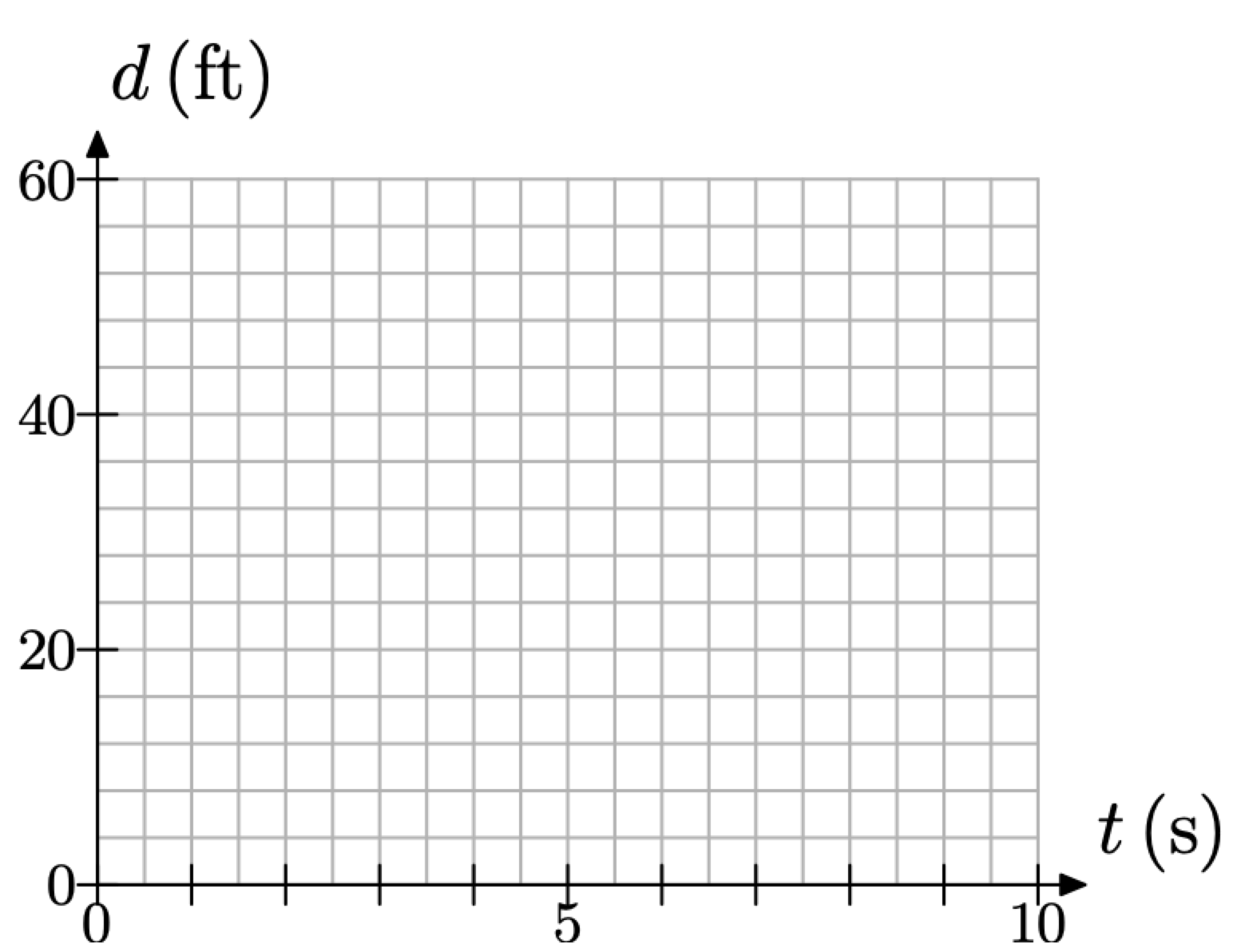
Figure \(\PageIndex{3}\). Scaling each axis to accommodate the rate.
At time t = 0, Sebastian is separated from his brother by a distance of d = 20 feet. This corresponds to the point (t, d) = (0, 20) shown in Figure \(\PageIndex{4}\)(a).
Next, Sebastian walks away from his brother at a constant rate of 4 feet per second. This means that for every second of time that elapses, the distance between the brothers increases by 4 feet. Starting at the point (0, 20), move 1 second (two boxes) to the right and 4 feet (1 box) upward to the point (1, 24), as shown in Figure \(\PageIndex{4}\)(b).
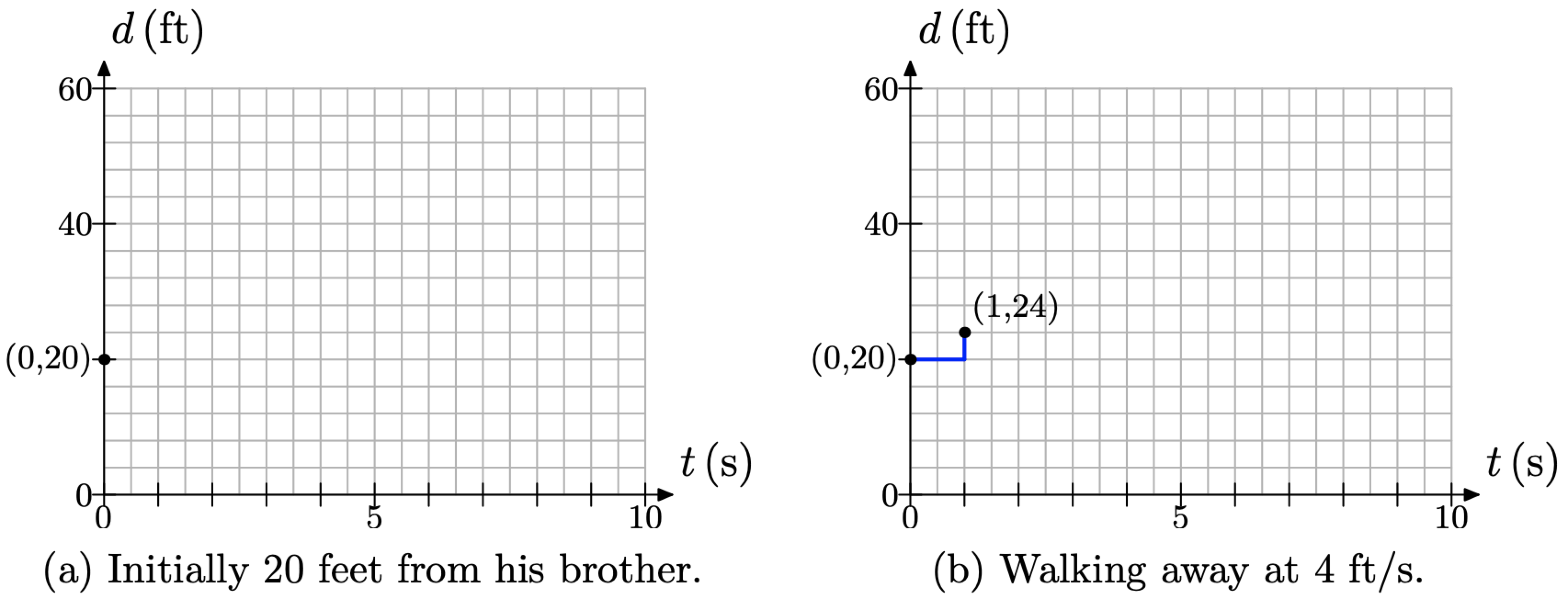
Figure \(\PageIndex{4}\).
The rate of separation is a constant 4 feet per second. So, continue indefinitely in the manner of Figure Figure \(\PageIndex{4}\)(b), moving 1 second (2 boxes) to the right, then 4 feet upward (1 box). This will produce the linear relationship between distance and time suggested in Figure \(\PageIndex{5}\)(a).
If we assume that the distance is a continuous function of time, a legitimate assumption due to the fact that the distance is increasing continuously at a constant rate of 4 feet per second, then we can replace the discrete set of data points in Figure \(\PageIndex{5}\)(a) with the line shown in Figure \(\PageIndex{5}\)(b).
The line in Figure \(\PageIndex{5}\)(b) is a continuous model. It can be drawn with a simple stroke of the pencil, without the tip of the pencil ever leaving contact with our graph paper. On the other hand, the set of points in Figure \(\PageIndex{4}\)(a) is a discrete model. After plotting a point, our pencil must break contact with our graph paper before plotting the next point. This is the essential difference between a discrete model and a continuous model.
In this case, the continuous model is a more accurate representation of the distance between the brothers. We say this because the distance between them is increasing at a constant rate of 4 feet per second, or 2 feet every half second, or 1 foot every quarter second, etc. Shortly, we will show an example where this sort of continuous model is unreasonable.
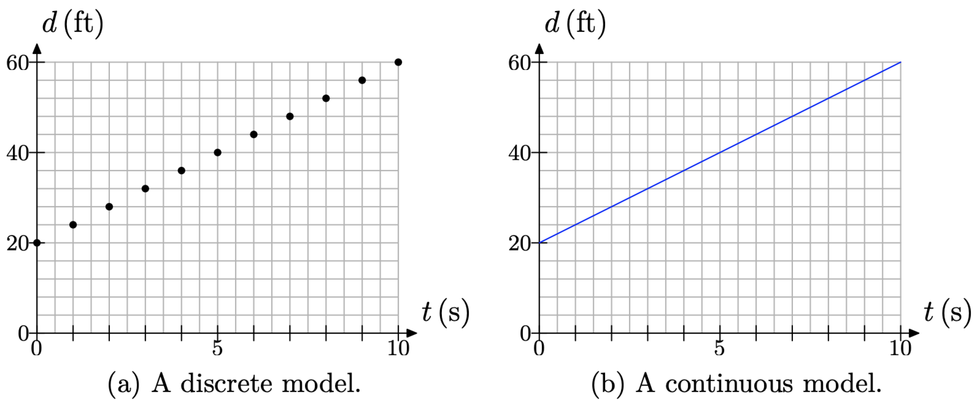
Figure \(\PageIndex{5}\). Constant rate yields a linear relationship.
Now that we’ve modeled the distance between the brothers with a graph, we can use the graph to make predictions. For example, to determine the distance between the brothers after 8 seconds, locate 8 seconds on the time axis, draw a vertical arrow to the line, then a horizontal arrow to the distance axis, as shown in Figure \(\PageIndex{6}\).
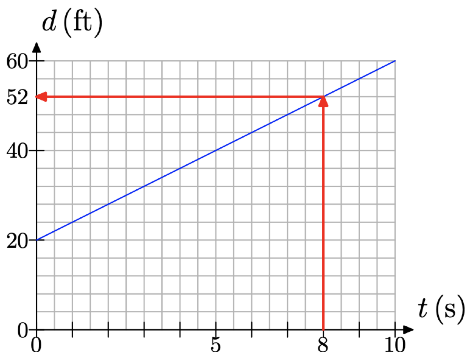
Figure \(\PageIndex{6}\). Predicting the distance between the brothers after 8 seconds.
However, suppose that we want to determine the distance between the brothers after 2 minutes. As the graph in Figure \(\PageIndex{5}\)(b) only models the distance over the first 10 seconds, we would have to redraw the graph over the first 2 minutes (120 seconds) to determine the answer. We did not plan ahead for this contingency, so perhaps we can model the distance between the brothers in another way, one that will more easily predict the distance between the brothers after an arbitrary amount of time t.
To this end, we search for a pattern that describes the distance d between the brothers as a function of time t. Because the distance between the brothers is increasing at a rate of 4 feet per second, we note that:
- At t = 0 seconds, the distance between the brothers is d = 20 feet.
- At t = 1 second, the distance between the brothers is d = 24 feet.
- At t = 2 seconds, the distance between the brothers is d = 28 feet.
- At t = 3 seconds, the distance between the brothers is d = 32 feet.
We summarize these results in Table \(\PageIndex{1}\)(a).
However, you don’t want to simplify the distances as we have in Table \(\PageIndex{1}\)(a), because you hide the pattern or the relationship between the distance d and the time t. It is more efficient to seek a relationship between distance and time in the following manner. After t = 1 second, the distance increases by 1 increment of 4 feet, so d = 20 + 4(1). After t = 2 seconds, the distance increases by 2 increments of 4 feet, so d = 20 + 4(2). Continuing in this manner, we have:
• At t = 3 seconds, the distance between the brothers is d = 20 + 4(3) feet.
• At t = 4 seconds, the distance between the brothers is d = 20 + 4(4) feet.
These results are summarized in Table \(\PageIndex{1}\)(b).
| t | d |
|---|---|
| 0 | 20 |
| 1 | 24 |
| 2 | 28 |
| 3 | 32 |
Table \(\PageIndex{1}\)(a) Determining a model equation.
| t | d |
|---|---|
| 0 |
20 |
| 1 | 20 + 4(1) |
| 2 | 20 + 4(2) |
| 3 | 20 + 4(3) |
Table \(\PageIndex{1}\)(b) Determining a model equation.
Unlike Table \(\PageIndex{1}\)(a), Table \(\PageIndex{1}\)(b) reveals a relationship between distance d and time t that can be described by the equation
\[d=20+4 t \nonumber \]
The careful reader will check that equation (3) reveals the correct distances for t = 0, 1, 2, and 3 seconds, as recorded in Table \(\PageIndex{1}\)(a). Two important observations can be made about equation (3).
- The 20 in d = 20 + 4t is the initial distance between the brothers and corresponds to the point (0, 20) in Figure \(\PageIndex{4}\)(a).
- The 4 in N = 20 + 4t is the rate at which the distance between the brothers is increasing (4 feet per second).
Moreover, equation (3) can be used to predict the distance between the brothers at 2 minutes. First, convert t = 2 minutes to t = 120 seconds, then substitute this number in our model equation (3).
\[d=20+4(120)=500 \nonumber \]
Thus, the distance between the brothers after 2 minutes is d = 500 feet.
We can also write the equation d = 20 + 4t using function notation.
\[d(t)=20+4 t \nonumber \]
Then, to find the distance between the brothers at the end of 2 minutes, we would perform the following calculation.
\[\begin{array}{l}{d(120)=20+4(120)} \\ {d(120)=500}\end{array} \nonumber \]
Unlike function notation, when the result is written d = 500 feet, note how one piece of information is hidden, namely the time. With function notation, we interpret d(120) = 500 to mean “the distance between the two brothers after 120 seconds is 500 feet.” Note how both the distance and the time are available in the notation d(120) = 500.
Modeling the Discrete with the Continuous
Jenny builds a rabbit hutch behind her barn. She places 25 rabbits in the hutch, then locks the door and leaves. Unfortunately, there is a flaw in the design of the hutch and the rabbits begin to escape at a constant rate of 5 rabbits every 2 hours. Again, we’ll model the number N of rabbits remaining in the hutch as a function of time t. First, we propose a graphical model.
Note that the number of rabbits remaining in the hutch depends on the amount of time that has passed. This makes the number N of rabbits remaining in the hutch the dependent variable, which we will place on the vertical axis in Figure \(\PageIndex{7}\)(a). Time t is the independent variable and is placed on the horizontal axis.
We’ll again choose a scale for our axes that accommodates the fact that the rabbit population is decreasing at a constant rate of 5 rabbits every 2 hours. In Figure \(\PageIndex{7}\)(b), we let each box on the vertical axis represent 1 rabbit, while two boxes on the horizontal axis represents 1 hour. We could just as easily let each box on the horizontal axis represent one hour, but our choice makes a graph that is a bit larger. Larger graphs are a bit easier to read and interpret.
At time t = 0 hours, the rabbit population is N = 25 rabbits. This fact is represented by the point (t, N) = (0, 25) in Figure \(\PageIndex{8}\)(a). Because the rabbit population decreases at a constant rate of 5 rabbits every 2 hours, we start at the point (0, 25), then move 2 hours (4 boxes) to the right, and 5 rabbits (5 boxes) down to the point (2, 20), also shown in Figure \(\PageIndex{8}\)(a).
The rate at which the rabbits are decreasing is constant at 5 rabbits every 2 hours, so continue indefinitely in the manner of Figure \(\PageIndex{8}\)(a), moving 2 hours (4 boxes) to the right, then 5 rabbits (5 boxes) downward. This will produce the linear relationship between the number of rabbits N and the time t shown in Figure \(\PageIndex{8}\)(b).
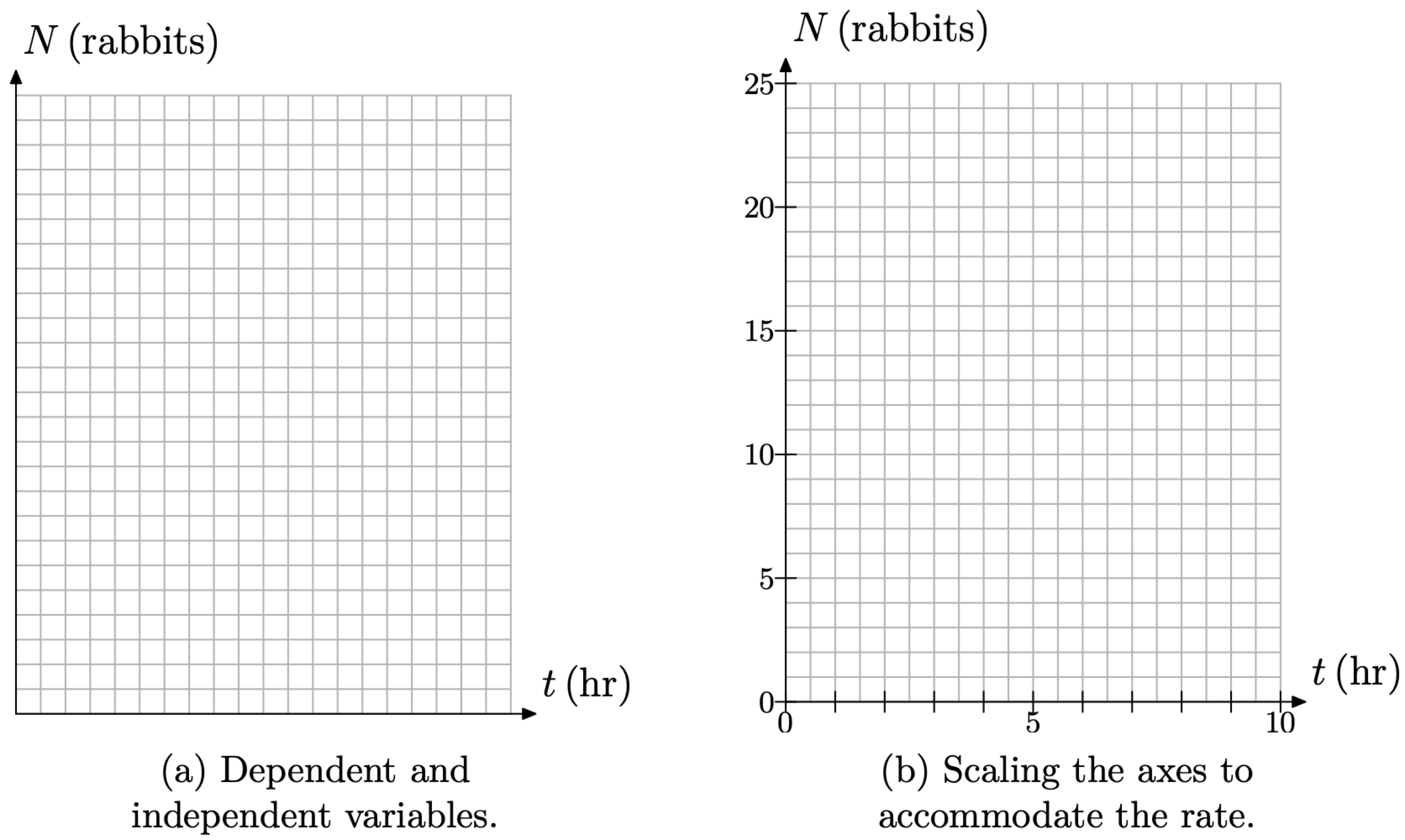
Figure \(\PageIndex{7}\).
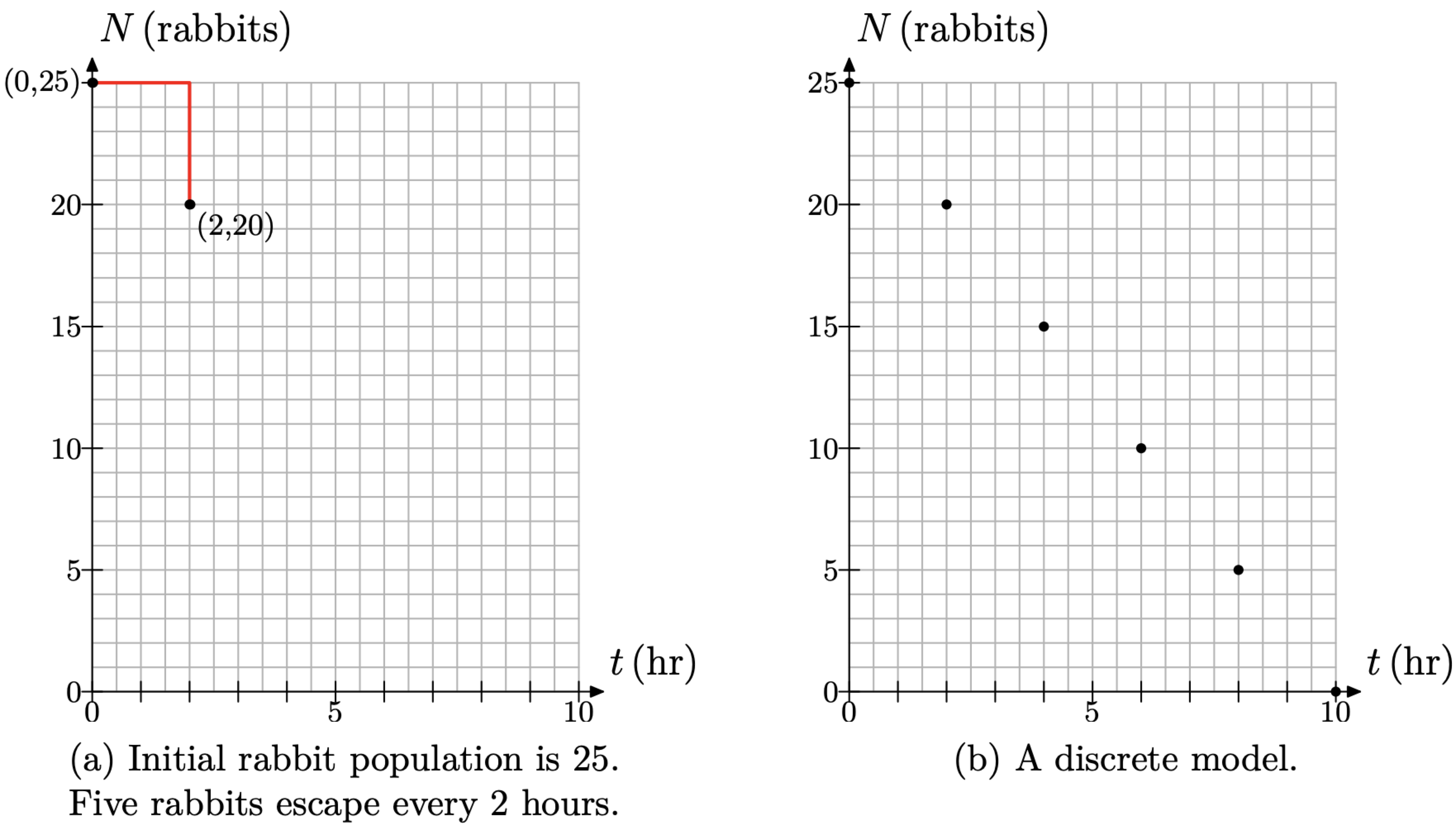
Figure \(\PageIndex{8}\).
We can draw a line through the data points in Figure \(\PageIndex{8}\)(b) to produce the continuous model in Figure \(\PageIndex{9}\)(a). However, we need to be aware of the shortcoming imposed by this continuous approximation. For example, consider the prediction in Figure \(\PageIndex{9}\)(b). Is it reasonable to say that 7.5 rabbits remain in the hutch after 7 hours?
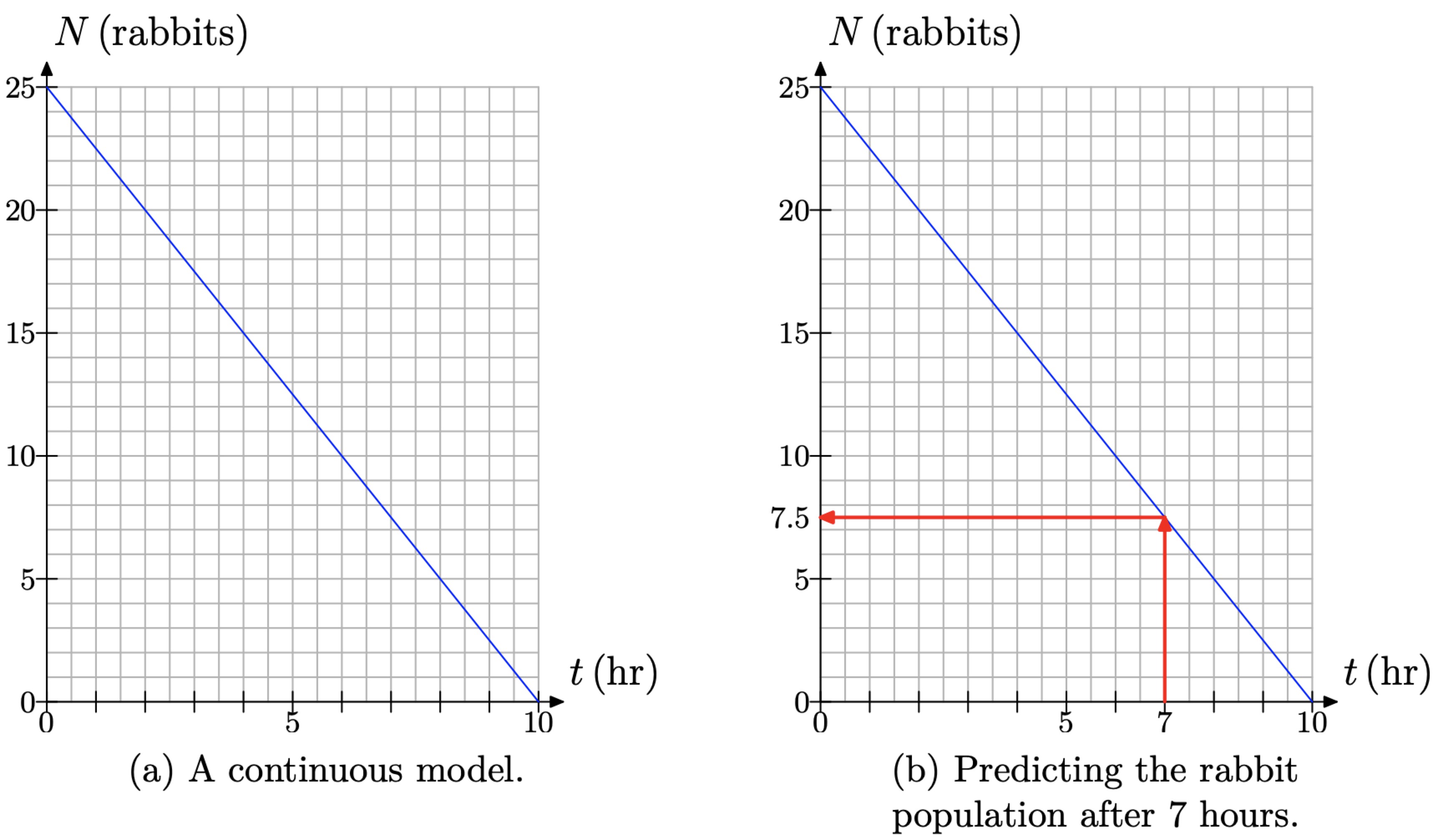
Figure \(\PageIndex{9}\).
In our first model, the distance between the brothers can be any real number, so a continuous model was appropriate. However, in the case of Jenny’s rabbit hutch, the remaining population must be a whole number of rabbits (unless a fox gets in), so modeling the population with the continuous line in Figure 9(b) is at best an approximation of reality. However, mathematicians will frequently model a discrete situation with a continuous model. As long as we are aware of its limitations, we can still use the model to make reasonable predictions. For example, we might say that there are approximately 7 rabbits left in the hutch after 7 hours.
We saw the advantage of using function notation at the end of our previous model, so let’s employ function notation a bit earlier in this model. We will let
\[N(t)=\text { the number of rabbits remaining after } t \text { hours. } \nonumber \]
Initially, at time t = 0, there are 25 rabbits in the hutch. Thus, we write
\[N(0)=25 \nonumber \]
It might be easier to think of losing 5 rabbits every 2 hours as being equivalent to losing “on average” 2.5 rabbits every hour. Thus, at the end of 1 hour, the number of rabbits decreases by one increment of 2.5 rabbits, and we write
\[N(1)=25-2.5(1) \nonumber \]
At the end of 2 hours, the rabbit population decreases by 2 increments of 2.5 rabbits and we can write
\[N(2)=25-2.5(2) \nonumber \]
At the end of 3 hours, the rabbit population decreases by 3 increments of 2.5 rabbits and we can write
\[N(3)=25-2.5(3) \nonumber \]
A clear pattern develops, particularly when we summarize these results in Table \(\PageIndex{2}\).
| t | N(t) |
|---|---|
| 0 | 25 |
| 1 | 25 − 2.5(1) |
| 2 | 25 − 2.5(2) |
| 3 | 25 − 2.5(3) |
Table \(\PageIndex{2}\) Determining a model equation.
Table \(\PageIndex{2}\) reveals a relationship between the number of rabbits N and time t that can be described by the equation \[N(t)=25-2.5 t \nonumber \]
\[N(t)=25-2.5 t \nonumber \]
The careful reader will again check that equation (4) returns the correct number of rabbits at times t = 0, 1, 2, and 3, as recorded in Table \(\PageIndex{2}\).
There are two important observations we can make about equation (4).
- The 25 in \(N(t) = 25 − 2.5t\) is the initial rabbit population and corresponds to the point (0, 25) in Figure \(\PageIndex{8}\)(a).
- The −2.5 in \(N(t) = 25−2.5t\) is the rate at which the rabbit population is decreasing “on average” (2.5 rabbits per hour).
The equation (4) can be used to predict the number of rabbits remaining in the hutch after t = 7 hours. Simply substitute t = 7 in equation (4).
\[N(7)=25-2.5(7)=7.5 \nonumber \]
It is important to note that the prediction made by the model equation is identical to that made by the model graph in Figure \(\PageIndex{9}\)(b).
However, again note that this equation is a continuous model, and its prediction that 7.5 rabbits remain in the hutch is not realistic (unless that fox got loose again). However, if we are aware of the model’s shortcomings, the equation can still be used as a good predictive tool. For example, we might again say that approximately 7 rabbits remain in the hutch after 7 hours. This can be written \(N(7) \approx 7\), which means that “after 7 hours, there are approximately 7 rabbits remaining in the hutch.”
Determining the Equation Model from the Graph
Mrs. Burke sets up a motion detector at the front of her classroom, then positions one of her students a fixed distance from the detector and asks the student to approach the detector at a constant speed. The detector measures the distance d (in meters) of the student from the detector as a function of time t (in seconds). The graph of distance d versus time t is given in Figure \(\PageIndex{10}\).
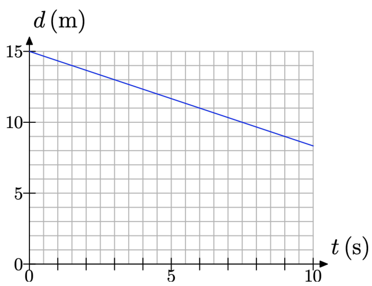
Figure \(\PageIndex{10}\). The detector measures the distance between student and detector versus time.
It is a simple matter to determine the student’s initial distance from the detector. We need only determine the value of d at time t = 0 seconds. The result is located at the point (0, 15), as shown in Figure \(\PageIndex{11}\)(a). Thus, the student sets up at an initial distance of 15 meters from the detector.
To determine the rate at which the student approaches the detector, we need to do a bit more work. Examine the graph and pick two points on the line. It makes things a bit easier if you pick points on the line that are situated at the intersection of two grid lines, but as we will show, this is not necessary. With this thought in mind, we’ve picked the points P(3, 13) and Q(6, 11) on the line, as shown in Figure \(\PageIndex{11}\)(b).
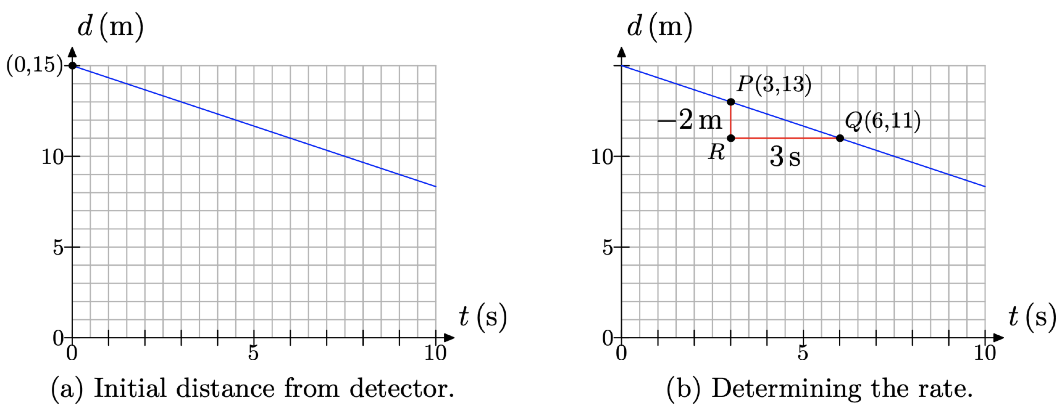
Figure \(\PageIndex{11}\). Determining initial distance and rate.
Draw a right triangle \(\triangle P Q R\) with sides parallel to the axes, as shown in Figure \(\PageIndex{11}\)(b). Determine the length of each side of the right triangle.
- Side PR is 2 boxes in length, but each box represents 1 meter, so side P R represents a decrease of 2 meters in distance from the detector. That is why we’ve used the minus sign in labeling the side PR with −2m in Figure \(\PageIndex{11}\)(b).
- Side RQ is 6 boxes in length, but 2 boxes represents 1 second, so side RQ represents an increase of 3 seconds in time. That is why we’ve labeled side RQ with 3 s in Figure \(\PageIndex{11}\)(b).
Thus, the distance between the student and detector is decreasing at a rate of 2 meters every 3 seconds.
What would happen if we picked two different points on the line? Consider the case in Figure \(\PageIndex{12}\), where we’ve picked the points on the line at P(3, 13) and Q(9, 9). We’ve also decided to draw right triangle \(\triangle P Q R\) on the opposite side of the line. However, note again that the sides of the right triangle \(\triangle P Q R\) are parallel to the horizontal and vertical axes.
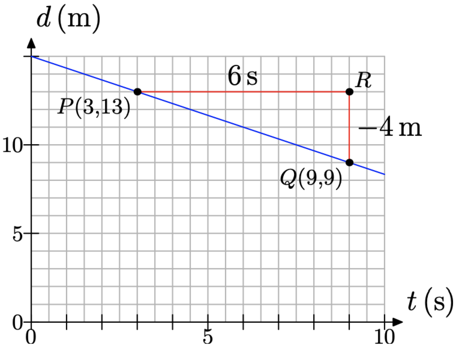
Figure \(\PageIndex{12}\). Determining the rate.
Determine the length of each side of triangle \(\triangle P Q R\).
- Side PR is 12 boxes in length, but 2 boxes represent 1 second, so side PR represents an increase of 6 seconds in time. That is why we’ve labeled side P R with 6 s in Figure \(\PageIndex{12}\).
- Side RQ is 4 boxes in length, but each box represents 1 meter, so side RQ represents a decrease of 4 meters in distance from the detector. That is why we’ve used a minus sign in labeling the side RQ with −4 m in Figure \(\PageIndex{12}\).
Thus, the distance between the student and detector is decreasing at a rate of 4 meters every 6 seconds. In symbols, we would write that the rate is
\[\text { Rate }=\frac{-4 \mathrm{m}}{6 \mathrm{s}}=-\frac{4}{6} \mathrm{m} / \mathrm{s} \nonumber \]
Note, however, that this reduces to \[\text { Rate }=-\frac{2}{3} \mathrm{m} / \mathrm{s} \nonumber \] which is identical to the rate found earlier when using the points P and Q in Figure \(\PageIndex{11}\)(b).
The fact that these rates are equivalent is due to the fact that the triangles (\triangle P Q R\) in Figure \(\PageIndex{11}\)(b) and Figure \(\PageIndex{12}\) are similar triangles, so their sides are proportional. Thus, it doesn’t matter which two points you pick on the line, nor does it matter which side of the line you place your right triangle. Thus, the only requirement is that you draw a right triangle with sides parallel to the coordinate axes.
Finally, let’s see if we can develop a model equation. We will define \[d(t)=\text { the distance from the detector at time } t \nonumber \]
Initially, the student is 15 meters from the detector. That is, at time t = 0, the distance from the detector is 15 meters. In symbols, we write
\[d(0)=15 \nonumber \]
The distance decreases at a rate of 2 meters every 3 seconds. This is equivalent to saying that the distance decreases 2/3 meters every second. At the end of 1 second, the distance has decreased by 1 increment of 2/3 meters, so the distance from the detector is given by
\[d(1)=15-\frac{2}{3}(1) \nonumber \]
At the end of 2 seconds, the distance has decreased by 2 increments of 2/3 meters, so the distance from the detector is given by
\[d(2)=15-\frac{2}{3}(2) \nonumber \]
At the end of 3 seconds, the distance has decreased by 3 increments of 2/3 meters, so the distance from the detector is given by
\[d(3)=15-\frac{2}{3}(3) \nonumber \]
A clear pattern emerges, particularly if you summarize the results as we have in Table \(\PageIndex{3}\).
| t | d(t) |
|---|---|
| 0 | 15 |
| 1 | 15 − (2/3)(1) |
| 2 | 15 − (2/3)(2) |
| 3 | 15 − (2/3)(3) |
Table \(\PageIndex{3}\) Determining a model equation.
Table \(\PageIndex{3}\) reveals that the linear relationship (see Figure \(\PageIndex{10}\)) between the distance d from the detector at time t can be modeled by the equation \[d(t)=15-\frac{2}{3} t \nonumber \]
Again, the careful reader will check that equation (5) returns the correct distance d at the times t = 0, 1, 2, and 3 recorded in Table \(\PageIndex{3}\).
There are two important observations to be made about equation (5).
1. The 15 in d(t) = 15−(2/3)t is the initial distance from the detector and corresponds to the point (0, 15) in Figure \(\PageIndex{11}\)(a).
2. The −2/3 in d(t) = 15−(2/3)t is the rate at which the distance between the student and detector is changing as determined in Figure \(\PageIndex{11}\)(b). It is negative because the distance is decreasing with time.
Equation (5) can be used to make predictions. For example, to determine the distance between the student and detector at the end of 9 seconds, insert t = 9 into equation (5).
\[d(9)=15-\frac{2}{3}(9)=15-6=9 \nonumber \]
Of course, the notation d(9) = 9 is interpreted to mean “the distance between the student and the detector after 9 seconds is 9 meters.


