
3.6: Chapter 3 Exercises with Solutions
- Page ID
- 24101
\( \newcommand{\vecs}[1]{\overset { \scriptstyle \rightharpoonup} {\mathbf{#1}} } \)
\( \newcommand{\vecd}[1]{\overset{-\!-\!\rightharpoonup}{\vphantom{a}\smash {#1}}} \)
\( \newcommand{\dsum}{\displaystyle\sum\limits} \)
\( \newcommand{\dint}{\displaystyle\int\limits} \)
\( \newcommand{\dlim}{\displaystyle\lim\limits} \)
\( \newcommand{\id}{\mathrm{id}}\) \( \newcommand{\Span}{\mathrm{span}}\)
( \newcommand{\kernel}{\mathrm{null}\,}\) \( \newcommand{\range}{\mathrm{range}\,}\)
\( \newcommand{\RealPart}{\mathrm{Re}}\) \( \newcommand{\ImaginaryPart}{\mathrm{Im}}\)
\( \newcommand{\Argument}{\mathrm{Arg}}\) \( \newcommand{\norm}[1]{\| #1 \|}\)
\( \newcommand{\inner}[2]{\langle #1, #2 \rangle}\)
\( \newcommand{\Span}{\mathrm{span}}\)
\( \newcommand{\id}{\mathrm{id}}\)
\( \newcommand{\Span}{\mathrm{span}}\)
\( \newcommand{\kernel}{\mathrm{null}\,}\)
\( \newcommand{\range}{\mathrm{range}\,}\)
\( \newcommand{\RealPart}{\mathrm{Re}}\)
\( \newcommand{\ImaginaryPart}{\mathrm{Im}}\)
\( \newcommand{\Argument}{\mathrm{Arg}}\)
\( \newcommand{\norm}[1]{\| #1 \|}\)
\( \newcommand{\inner}[2]{\langle #1, #2 \rangle}\)
\( \newcommand{\Span}{\mathrm{span}}\) \( \newcommand{\AA}{\unicode[.8,0]{x212B}}\)
\( \newcommand{\vectorA}[1]{\vec{#1}} % arrow\)
\( \newcommand{\vectorAt}[1]{\vec{\text{#1}}} % arrow\)
\( \newcommand{\vectorB}[1]{\overset { \scriptstyle \rightharpoonup} {\mathbf{#1}} } \)
\( \newcommand{\vectorC}[1]{\textbf{#1}} \)
\( \newcommand{\vectorD}[1]{\overrightarrow{#1}} \)
\( \newcommand{\vectorDt}[1]{\overrightarrow{\text{#1}}} \)
\( \newcommand{\vectE}[1]{\overset{-\!-\!\rightharpoonup}{\vphantom{a}\smash{\mathbf {#1}}}} \)
\( \newcommand{\vecs}[1]{\overset { \scriptstyle \rightharpoonup} {\mathbf{#1}} } \)
\(\newcommand{\longvect}{\overrightarrow}\)
\( \newcommand{\vecd}[1]{\overset{-\!-\!\rightharpoonup}{\vphantom{a}\smash {#1}}} \)
\(\newcommand{\avec}{\mathbf a}\) \(\newcommand{\bvec}{\mathbf b}\) \(\newcommand{\cvec}{\mathbf c}\) \(\newcommand{\dvec}{\mathbf d}\) \(\newcommand{\dtil}{\widetilde{\mathbf d}}\) \(\newcommand{\evec}{\mathbf e}\) \(\newcommand{\fvec}{\mathbf f}\) \(\newcommand{\nvec}{\mathbf n}\) \(\newcommand{\pvec}{\mathbf p}\) \(\newcommand{\qvec}{\mathbf q}\) \(\newcommand{\svec}{\mathbf s}\) \(\newcommand{\tvec}{\mathbf t}\) \(\newcommand{\uvec}{\mathbf u}\) \(\newcommand{\vvec}{\mathbf v}\) \(\newcommand{\wvec}{\mathbf w}\) \(\newcommand{\xvec}{\mathbf x}\) \(\newcommand{\yvec}{\mathbf y}\) \(\newcommand{\zvec}{\mathbf z}\) \(\newcommand{\rvec}{\mathbf r}\) \(\newcommand{\mvec}{\mathbf m}\) \(\newcommand{\zerovec}{\mathbf 0}\) \(\newcommand{\onevec}{\mathbf 1}\) \(\newcommand{\real}{\mathbb R}\) \(\newcommand{\twovec}[2]{\left[\begin{array}{r}#1 \\ #2 \end{array}\right]}\) \(\newcommand{\ctwovec}[2]{\left[\begin{array}{c}#1 \\ #2 \end{array}\right]}\) \(\newcommand{\threevec}[3]{\left[\begin{array}{r}#1 \\ #2 \\ #3 \end{array}\right]}\) \(\newcommand{\cthreevec}[3]{\left[\begin{array}{c}#1 \\ #2 \\ #3 \end{array}\right]}\) \(\newcommand{\fourvec}[4]{\left[\begin{array}{r}#1 \\ #2 \\ #3 \\ #4 \end{array}\right]}\) \(\newcommand{\cfourvec}[4]{\left[\begin{array}{c}#1 \\ #2 \\ #3 \\ #4 \end{array}\right]}\) \(\newcommand{\fivevec}[5]{\left[\begin{array}{r}#1 \\ #2 \\ #3 \\ #4 \\ #5 \\ \end{array}\right]}\) \(\newcommand{\cfivevec}[5]{\left[\begin{array}{c}#1 \\ #2 \\ #3 \\ #4 \\ #5 \\ \end{array}\right]}\) \(\newcommand{\mattwo}[4]{\left[\begin{array}{rr}#1 \amp #2 \\ #3 \amp #4 \\ \end{array}\right]}\) \(\newcommand{\laspan}[1]{\text{Span}\{#1\}}\) \(\newcommand{\bcal}{\cal B}\) \(\newcommand{\ccal}{\cal C}\) \(\newcommand{\scal}{\cal S}\) \(\newcommand{\wcal}{\cal W}\) \(\newcommand{\ecal}{\cal E}\) \(\newcommand{\coords}[2]{\left\{#1\right\}_{#2}}\) \(\newcommand{\gray}[1]{\color{gray}{#1}}\) \(\newcommand{\lgray}[1]{\color{lightgray}{#1}}\) \(\newcommand{\rank}{\operatorname{rank}}\) \(\newcommand{\row}{\text{Row}}\) \(\newcommand{\col}{\text{Col}}\) \(\renewcommand{\row}{\text{Row}}\) \(\newcommand{\nul}{\text{Nul}}\) \(\newcommand{\var}{\text{Var}}\) \(\newcommand{\corr}{\text{corr}}\) \(\newcommand{\len}[1]{\left|#1\right|}\) \(\newcommand{\bbar}{\overline{\bvec}}\) \(\newcommand{\bhat}{\widehat{\bvec}}\) \(\newcommand{\bperp}{\bvec^\perp}\) \(\newcommand{\xhat}{\widehat{\xvec}}\) \(\newcommand{\vhat}{\widehat{\vvec}}\) \(\newcommand{\uhat}{\widehat{\uvec}}\) \(\newcommand{\what}{\widehat{\wvec}}\) \(\newcommand{\Sighat}{\widehat{\Sigma}}\) \(\newcommand{\lt}{<}\) \(\newcommand{\gt}{>}\) \(\newcommand{\amp}{&}\) \(\definecolor{fillinmathshade}{gray}{0.9}\)3.1 Exercises

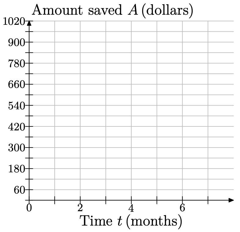
Jodiah is saving his money to buy a Playstation 3 gaming system. He estimates that he will need $950 to buy the unit itself, accessories, and a few games. He has $600 saved right now, and he can reasonably put $60 into his savings at the end of each month. Since the amount of money saved depends on how many months have passed, choose time, in months, as your independent variable and place it on the horizontal axis. Let t represent the number of months passed, and make a mark for every month. Choose money saved, in dollars, as your dependent variable and place it on the vertical axis. Let A represent the amount saved in dollars. Since Jodiah saves $60 each month, it will be convenient to let each box represent $60. Copy the following coordinate system onto a sheet of graph paper.
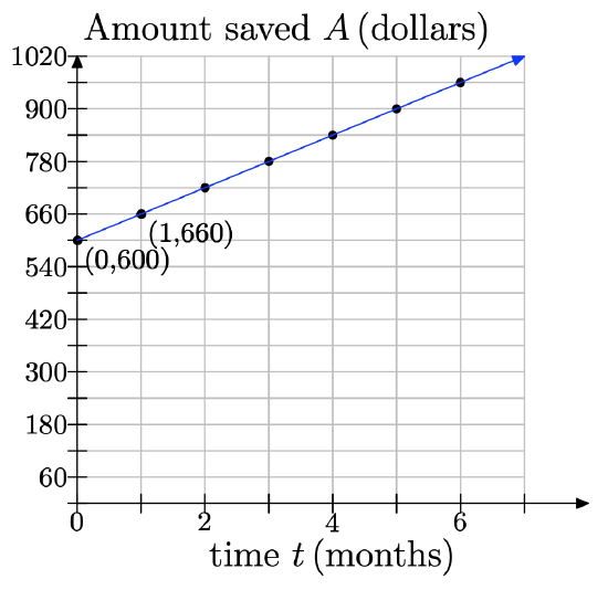
a) At month 0, Jodiah has $600 saved. This corresponds to the point (0, 600). Plot this point on your coordinate system.
b) For the next month, he saved $60 more. Beginning at point (0, 600), move 1 month to the right and $60 up and plot a new data point. What are the coordinates of this point?
c) Each time you go right 1 month, you must go up by $60 and plot a new data point. Repeat this process until you reach the edge of the coordinate system.
d) Keeping in mind that we are modeling this discrete situation continuously, draw a line through your data points.
e) Use your graph to estimate how much money Jodiah will have saved after 7 months. f) Using your graph, estimate how many months it will take him to have saved up enough money to buy his gaming system, accessories, and games.
- Answer
-
d)
e)
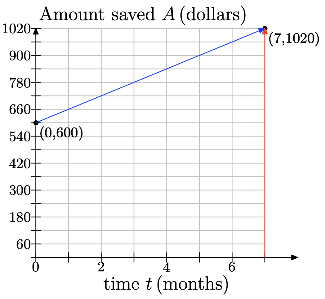
From the graph, when t = 7 months, he will have saved $1020.
f)
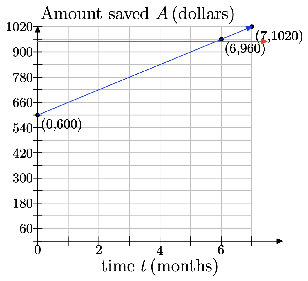
Note that we’ve modeled a discrete problem continuously: He saves $60 at the end of each month, and he will have $900 by the end of month five; and then $960 by the end of month six. There will be no time at which he has exactly $950, so the answer is 6 months, at which point he’ll have $960.

The sign above shows the prices for a taxi ride from Liberty Cab Company. Since the cost depends on the distance traveled, make the distance be the independent variable and place it on the horizontal axis. Let d represent the distance traveled, in miles. Because the cab company charges per 1/6 mile, it is convenient to mark every 1/6 mile. Make price, in $, your dependent variable and place it on the vertical axis. Let C represent the cost, in $. Because the cost occurs in increments of 40c, mark every 40c along the vertical axis. Copy the following coordinate system onto a sheet of graph paper.
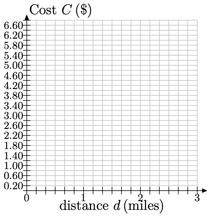
a) For the first 1/6 mile of travel, the cost is $2.30. This corresponds to the point (1/6,$2.30). Plot this point on your coordinate system.
b) For the next 1/6 of a mile, the cost goes up by 40\(\cent\). Beginning at point (1/6,$2.30), move 1/6 of a mile to the right and 40c up and plot a new data point. What are the coordinates of this point?
c) Each time you go right 1/6 of a mile, you must go up by 40\(\cent\) and plot a new data point. Repeat this process until you reach the edge of your coordinate system.
d) Keeping in mind that we are modeling this discrete situation continuously, draw a line through your data points.
e) Melissa steps into a cab in the city of Niagara Falls, about 2 miles from Niagara Falls State Park. Use your graph to estimate the fare to the park.
f) Elsewhere in the area, Georgina takes a cab. She has only $5 for the fare. Use the graph to estimate how far she can travel, in miles, with only $5 for the fare.
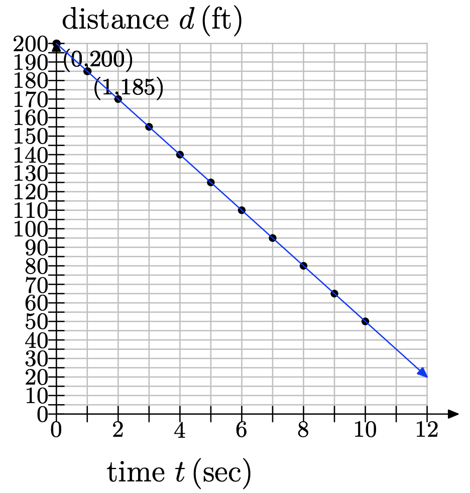
A boat is 200 ft from a buoy at sea. It approaches the buoy at an average speed of 15 ft/s.
a) Choosing time, in seconds, as your independent variable and distance from the buoy, in feet, as your dependent variable, make a graph of a coordinate system on a sheet of graph paper showing the axes and units. Use tick marks to identify your scales.
b) At time t=0, the boat is 200 ft from the buoy. To what point does this correspond? Plot this point on your coordinate system.
c) After 1 second, the boat has drawn 15 ft closer to the buoy. Beginning at the previous point, move 1 second to the right and 15 ft down (since the distance is decreasing) and plot a new data point. What are the coordinates of this point?
d) Each time you go right 1 second, you must go down by 15 ft and plot a new data point. Repeat this process until you reach 12 seconds.
e) Draw a line through your data points.
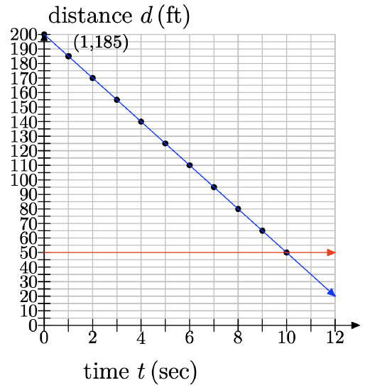
f) When the boat is within 50 feet of the buoy, the driver wants to begin to slow down. Use your graph to estimate how soon the boat will be within 50 feet of the buoy.
- Answer
-
e)
f) We draw a line at 50 ft and see that it occurs at 10 seconds:
Joe owes $24,000 in student loans. He has finished college and is now working. He can afford to pay $1500 per month toward his loans.
a) Choose time in months as your independent variable and amount owed, in $, as the dependent variable. On a sheet of graph paper, make a sketch of the coordinate system, using tick marks and labeling the axes appropriately.
b) At time t = 0, Joe has not yet paid anything toward his loans. To what point does this correspond? Plot this point on your coordinate system.
c) After one month, he pays $1500. Beginning at the previous point, move 1 month to the right and $1500 down (down because the debt is decreasing). Plot this point. What are its coordinates?
d) Each time you go 1 month to the right, you must move $1500 down. Continue doing this until his loans have been paid off.
e) Keeping in mind that we are modeling this discrete situation continuously, draw a line through your data points.
f) Use the graph to determine how many months it will take him to pay off the full amount of his loans.

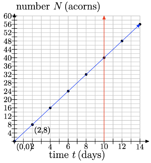
Earl the squirrel has only ten more days until hibernation. He needs to save 50 more acorns. He is tired of collecting acorns and so he is only able to gather 8 acorns every 2 days.
a) Let t represent time in days and make it your independent variable. Let N represent the number of acorns collected and make it your dependent variable. Set up an appropriately scaled coordinate system on a sheet of graph paper.
b) At time t = 0, Earl has collected zero of the acorns he needs. To what point does this correspond? Plot this point on your coordinate system.
c) After two days (t = 2), Earl has collected 8 acorns. Beginning at the previous point, move 2 days to the right and 8 acorns up. Plot this point. What are its coordinates?
d) Each time you go 2 days to the right, you must move 8 acorns up and plot a point. Continue doing this until you reach 14 days.
e) Keeping in mind that we are modeling this discrete situation continuously, draw a line through your data points.
f) Use the graph to determine how many acorns he will have collected after 10 days. Will Earl have collected enough acorns for his winter hibernation?
g) Notice that the number of acorns collected is increasing at a rate of 8 acorns every 2 days. Reduce this to a rate that tells the average number of acorns that is collected each day.
h) The table below lists the number of acorns Earl will have collected at various times. Some of the entries have been completed for you. For example, at t = 0, Earl has no acorns, so N = 0. After one day, the amount increases by 4, so N = 0 + 4(1). After two days, two increases have occurred, so N = 0+4(2). The pattern continues. Fill in the missing entries.
| t | N |
|---|---|
| 0 | 0 |
| 1 | 0 + 4(1) |
| 2 | 0 + 4(2) |
| 3 | 0 + 4(3) |
| 4 | |
| 6 | |
| 8 | |
| 10 | |
| 12 | |
| 14 |
i) Express the number of acorns collected, N, as a function of the time t, in days.
j) Use your function to predict the number of acorns that Earl will have after 10 days. Does this answer agree with your estimate from part (f)?
- Answer
-
e)
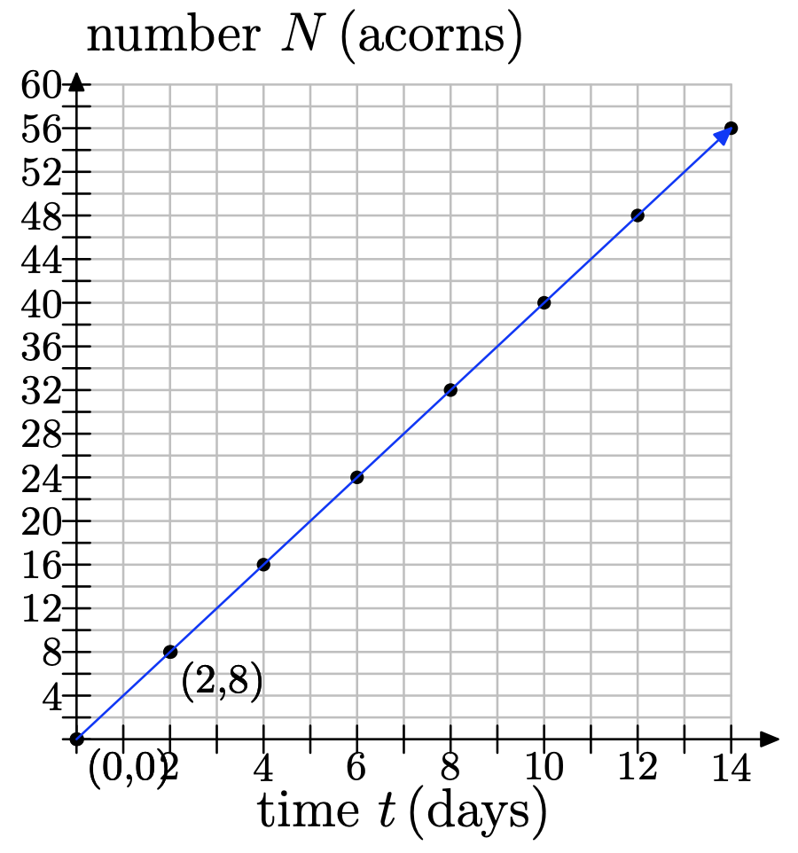
f) If you draw a line at 10 days, then you can see that he will have collected 40 acorns.
g) \(\frac{8}{2}\) acorns/day = 4 acorns/day
h) Following the pattern, we get:
t N 0 0 1 0 + 4(1) 2 0 + 4(2) 3 0 + 4(3) 4 0+4(4) 6 0+4(6) 8 0+4(8) 10 0+4(10) 12 0+4(12) 14 0+4(14)
i) N = 0 + 4t or N = 4t
j) At t = 10, N = 0 + 4(10) = 40 acorns.
On network television, a typical hour of programming contains 15 minutes of commercials and advertisements and 45 minutes of the program itself.
a) Choose amount of television watched as your independent variable and place it on the horizontal axis. Let T represent the amount of television watched, in hours. Choose total amount of commercials/ads watched as your dependent variable and place it on the vertical axis. Let C represent the total amount of commercials/ads watched, in minutes. Using a sheet of graph paper, make a sketch of a coordinate system and label appropriately.
b) For 0 hours of programming watched, 0 minutes of commercials have been watched. To what point does this correspond? Plot it on your coordinate system.
c) After watching 1 hour of program-ming, 15 minutes of commercials/ads have been watched. Beginning at the previous point, move 1 hour to the right and 15 minutes up. Plot this point. What are its coordinates?
d) Each time you go 1 hour to the right, you must move 15 minutes up and plot a point. Continue doing this until you reach 5 hours of programming.
e) Draw a line through your data points.
f) Billy watches TV for five hours on Monday. Use the graph to determine how many minutes of commercials he has watched during this time.
g) Suppose a person has watched one hour of commercials/ads. Use the graph to estimate how many hours of television he watched.
h) The following table shows numbers of hours of programming watched as it relates to number of minutes of commercials/ads watched. For 0 hours of TV, 0 minutes of commercials/ads are watched. For each hour of TV watched, we must count 15 minutes of commercials/ads. So, for 1 hour, 0 + 15(1) minutes of commercials are watched. For 2 hours, 0 + 15(2) minutes; and so on. Fill in the missing entries.
| T (hrs) | C (mins) |
|---|---|
| 0 | 0 |
| 1 | 0 + 15(1) |
| 2 | 0 + 15(2) |
| 3 | |
| 4 | |
| 5 |
i) Express the amount of commercials/ads watched, C, as a function of the amount of television watched T. Use your equation to predict the amount of commercials/ads watched for 5 hours of television programming. Does this answer agree with your estimate from part (f)?
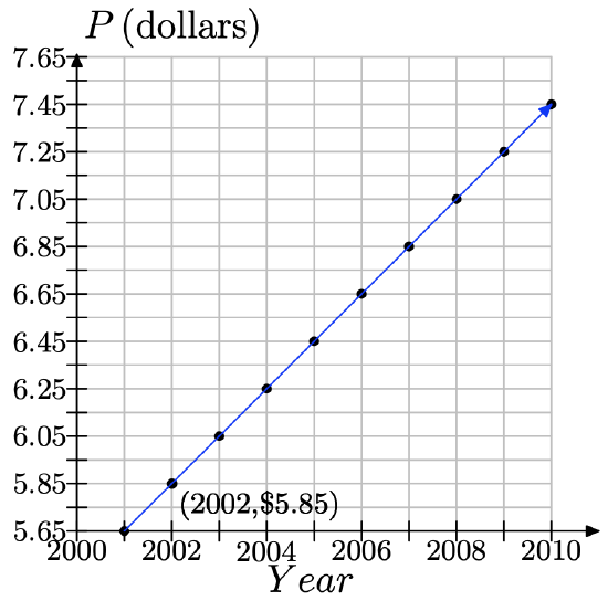
According to NATO (the National Association of Theatre Owners), the average price of a movie ticket was 5.65 dollars in the year 2001. Since then, the average price has been rising each year by about 20\(\cents\).
a) Choose year, beginning with 2000, as the independent variable and make marks every year on the axis. Choose average ticket price, in dollars, as your dependent variable and begin at 5.65 dollars, with marks every 10\(\cents\) above. Make a sketch of a coordinate system and label appropriately.
b) In 2001, the average ticket price was 5.65 dollars, corresponding to the point (2001, 5.65). Plot it on your coordinate system.
c) In 2002, one year later, the average price rose by about 20\(\cents\). Beginning at the previous point, move right by 1 year and up by 20\(\cents\) and plot the point. What are its coordinates?
d) Each time you go 1 year to the right, you must move up by 20\(\cents\) and plot a point. Continue doing this until the year 2010.
e) Keeping in mind that we are modeling this discrete situation continuously, draw a line through your data points.
f) Use the graph to estimate what year the average price of a ticket will pass 7.00 dollars.
- Answer
-
e)
f) Draw a line for $7.00 and look for the year.
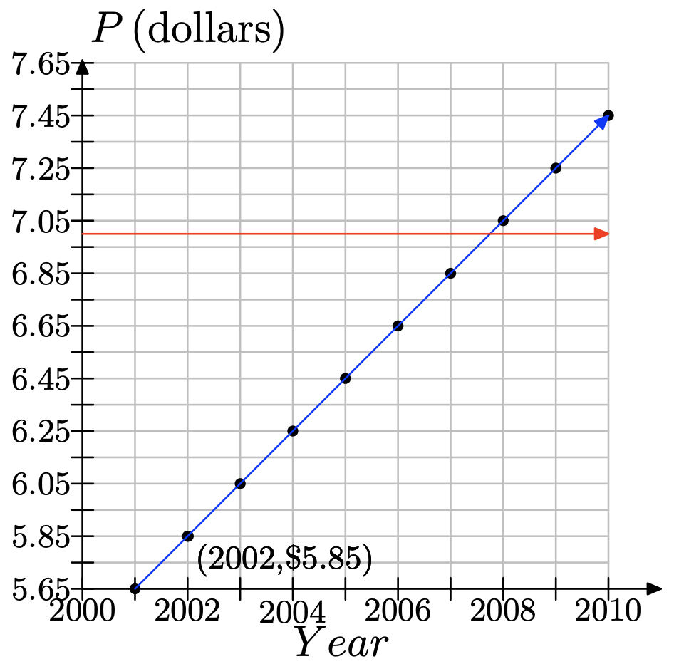
Notice that year is between 2007 and 2008. But this is a discrete problem, since we are only dealing with whole years. Thus, the answer is 2008.
When Jessica drives her car to a work-related conference, her employer reimburses her approximately 45 cents per mile to cover the cost of gas and the wear-and-tear on the vehicle.
a) Using distance traveled d, in miles, as the independent variable and amount reimbursed A, in dollars, as the dependent variable, make a sketch of a coordinate system and label appropriately. Mark distance every 5 miles and amount reimbursed every $0.45.
b) For traveling 0 miles, the reimbursement is 0. This corresponds to the point (0, 0). Plot it on your coordinate system.
c) For a trip that requires her to drive a total of 5 miles, she is reimbursed 5(0.45) = $2.25. This corresponds to the point (5, $2.25). Plot it.
d) For each 5 miles you go to the right, you must go up $2.25 and plot the point. Do this until you reach 20 miles.
e) Keeping in mind that we are modeling this discrete situation continuously, draw a line through your data points.
f) In March, Jessica attends a conference that is only 5 miles away. Counting round trip, she travels 10 total miles. Use the graph to determine how much she is reimbursed.
g) In December, she attends a conference 10 miles away. How long is her trip in total? Use the graph to determine how much she will be reimbursed.
h) For longer trips, such as 200 total miles, you will probably need to make a much larger graph. And what if she travels 400 miles? Or further? It is limitations such as these that make it useful to find an equation that describes what the graph shows. To find the equation, we start with a table that helps us to understand the relationship between the dependent and independent variables. Complete the table below.
| d (miles) | A ($) |
|---|---|
| 0 | 0 |
| 1 | 0 + 0.45(1) |
| 2 | 0 + 0.45(2) |
| 3 | |
| 4 | |
| 5 | |
| 10 | |
| 20 | |
| 50 | |
| 100 |
i) Use the table from part (h) to come up with an equation that relates d and A.
j) Now, use the equation to determine the reimbursement amounts for trips of 200 miles and 400 miles.
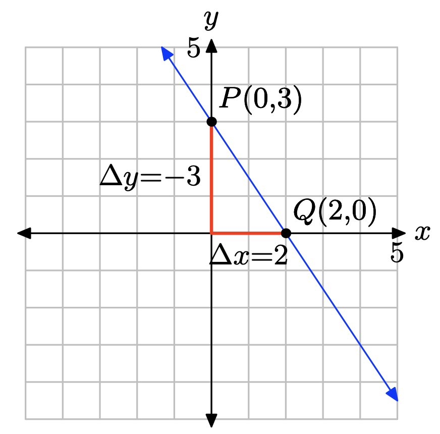
Temperature is typically measured in degrees Fahrenheit in the United States; but it is measured in degrees Celsius in many other countries. The relationship between Fahrenheit and Celsius is linear. Let’s choose the measurement of degrees in Celsius to be our independent variable and the measurement of degrees in Fahrenheit to be our dependent variable. Water freezes at 0 degrees Celsius, which corresponds to 32 degrees Fahrenheit; and water boils at 100 degrees Celsius, which corresponds to 212 degrees Fahrenheit. We can plot this information as the two points (0,32) and (100,212). The relationship is linear, so have the following graph:
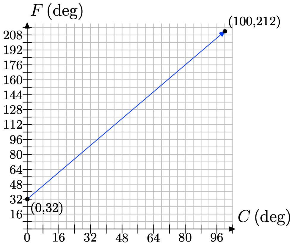
a) Use the graph to approximate the equivalent Fahrenheit temperature for 48 degree Celsius.
b) To determine the rate of change of Fahrenheit with respect to Celsius, we draw a right triangle with sides parallel to the axes that connects the two points we know...
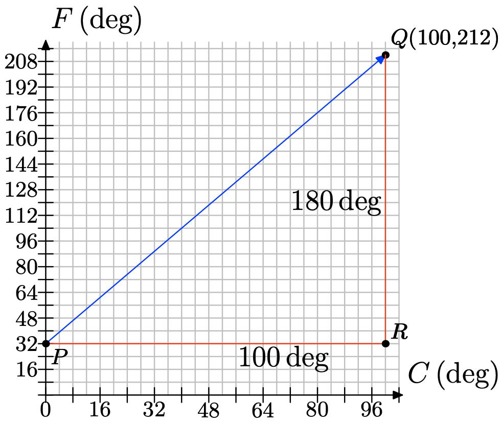
Side PR is 100 degrees long, representing an increase in 100 degrees Celsius. Side RQ is 180 degrees, representing an increase in 180 degrees Fahrenheit. Find the rate of increase of Fahrenheit per Celsius. c) The following table shows some values of temperatures in Celsius and their corresponding Fahrenheit readings. Zero degrees Celsius corresponds to 32 degrees Fahrenheit. Our rate is 9 degrees Fahrenheit for every 5 degrees Celsius, or 9/5 of a degree Fahrenheit for every 1 degree Celsius. So, for 1 degree Celsius, we increase the Fahrenheit reading by 9/5 degree, getting 32 + 9/5(1). For 2 degrees Celsius, we increase by two occurrences of 9/5 degree to get 32 + 9/5(2). Fill in the missing entries, following the pattern.
| C (deg) | F (deg) |
|---|---|
| 0 | 32 |
| 1 | \(32 + \frac{9} {5} (1)\) |
| 2 | \(32 + \frac{9} {5} (2)\) |
| 3 | \(32 + \frac{9} {5} (3)\) |
| 4 | |
| 5 | |
| 10 | |
| 20 | |
| 48 | |
| 100 |
d) Use the table to form an equation that gives degrees Fahrenheit in terms of degrees Celsius.
- Answer
-
a) We make a line at 48 degrees Celsius and read off the Fahrenheit estimate.
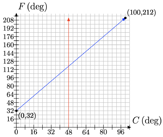
The estimate should be approximately 120 degrees Fahrenheit.
b) \(\dfrac{changeinF}{ changeinC} = \dfrac{180}{ 100 }= \dfrac{9}{ 5}\)
c)
C (deg) F (deg) 0 32 1 \(32 + \frac{9} {5} (1)\) 2 \(32 + \frac{9} {5} (2)\) 3 \(32 + \frac{9} {5} (3)\) 4 \(32 + \frac{9} {5} (4)\) 5 \(32 + \frac{9} {5} (5)\) 10 \(32 + \frac{9} {5} (10)\) 20 \(32 + \frac{9} {5} (20)\) 48 \(32 + \frac{9} {5} (48)\) 100 \(32 + \frac{9} {5} (100)\)
d) F = 9 5C + 32
On June 16, 2006, the conversion rate from Euro to U.S. dollars was approximately 0.8 to 1, meaning that every 0.8 Euros were worth 1 U.S. dollar.
a) Choosing dollars to be the independent variable and Euros to be the dependent variable, make a graph of co-ordinate system. Mark every dollar on the dollar axis and every 0.8 Euros on the Euro axis. Label appropriately.
b) Zero dollars are worth 0 Euros. This corresponds to the point (0, 0). Plot it on your coordinate system.
c) One dollar is worth 0.8 Euros. Plot this as a point on your coordinate system.
d) For every dollar you move to the right, you must go up 0.8 Euros and plot a point. Do this until you reach $10.
e) Draw a line through your data points.
f) Use the graph to estimate how many Euros $8 are worth.
g) Use the graph to estimate how many dollars 5 Euros are worth.
h) The following table shows some values of dollars and their corresponding value in Euros. Fill in the missing entries.
| Dollars | Euros |
|---|---|
| 0 | 0 |
| 1 | 0 + 0.8(1) |
| 2 | 0 + 0.8(2) |
| 3 | |
| 4 | |
| 5 | |
| 10 |
i) Use the table to make an equation that can be used to convert dollars to Euros.
j) Use the equation from (i) to convert $8 to Euros. Does your answer agree with the answer from (f) that you obtained using the graph?
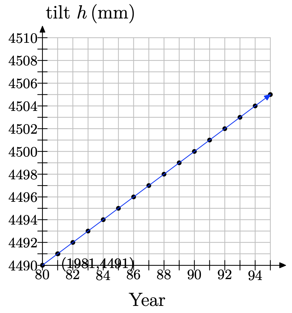
The Tower of Pisa in Italy has its famous lean to the south because the clay and sand ground on which it is built is softer on the south side than the north. The tilt is often found by measuring the distance that the upper part of the tower overhangs the base, indicated by h in the figure below. In 1980, the tower had a tilt of h = 4.49m, and this tilt was increasing by about 1 mm/year.

Figure \(\PageIndex{1}\). h measures the tilt of the Tower of Pisa.
We will investigate how the tilt of the tower changed from 1980 to 1995.
a) First, note that our units do not match: The tilt in 1980 was given as 4.49 m, but the annual increase in the tilt is given as 1 mm/year. Our first goal is to make the units the same. We will use millimeters (mm). Convert 4.49 m to mm.
b) Get a sheet of graph paper. Since the tilt of the tower depends on the year, make the year the independent variable and place it on the horizontal axis. Let t represent the year. Make the tilt the dependent variable and place it on the vertical axis. Let h represent the tilt, measured in millimeters (mm). Choose 1980 as the first year on the horizontal axis and mark every year thereafter, until 1995. Let the vertical axis begin at 4.49 m, converted to mm from part (a), since that was our first measurement; and then we mark every 1 mm thereafter up to 4510 mm.
c) Think of 1980 as the starting year. Together with the tilt measurement from that year, it forms a point. What are the coordinates of this point? Plot the point on your coordinate system.
d) Beginning at the first point, from part (c), move one year to the right (to 1981) and 1 mm up (because the tilt increases) and plot a new data point.
e) Each time you move one year to the right, you must move 1 mm up and plot a new point. Repeat this process until you reach the year 1995.
f) Keeping in mind that we are modeling this discrete situation continuously, draw a line through your data points. We can use this model to make predictions.
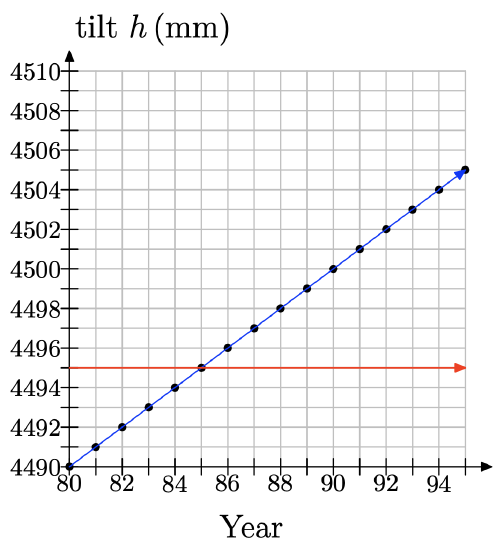
g) According to computer simulation models, which use sophisticated mathematics, the tower would be in danger of collapsing when h reaches about 4495 mm. Use your graph to estimate what year this would happen.
h) In reality, the tilt of the tower passed 4495 mm and the tower did not collapse. In fact, the tilt increased to 4500 mm before the tower was closed on January 7, 1990, to undergo renovations to decrease the tilt. (The tower was reopened in 2001, after engineers used weights and removed dirt from under the base to decrease the tilt by 450 mm.) What might be some reasons why the prediction of the computer model was wrong?
i) The following table lists the tilt of the tower, h, the year, and the number of years since 1980. In 1980, the tilt was 4490 mm and no occurrences of the 1 mm increase had happened yet, so we fill in 4490 + 0(1) = 4490. In 1981, one occurrence of the 1 mm increase had occurred because one year had passed since 1980. Therefore, the tilt was 4490 + 1(1). In 1982, two occurrences of the 1 mm increase had occurred, because 2 years had passed since 1980. Thus, the tilt was 4490 + 2(1). And the pattern continues in this manner. Fill in the remaining entries.
| Year | yrs x after ’80 | tilt h |
|---|---|---|
| 1980 | 0 | 4490 + 0(1) |
| 1981 | 1 | 4490 + 1(1) |
| 1982 | 2 | 4490 + 2(1) |
| 1983 | ||
| 1984 | ||
| 1985 | ||
| 1986 | ||
| 1987 | ||
| 1988 | ||
| 1989 | ||
| 1990 | ||
| 1991 | ||
| 1992 | ||
| 1993 | ||
| 1994 | ||
| 1995 |
j) Let x represent the number of years since 1980 and h represent the tilt. Using the table above, write an equation that relates h and x.
k) Use your equation to predict the tilt in 1990. Does it agree with the actual value from 1990? Does it agree with the value that is shown on the graph you made?
l) In part (g), you used the graph to predict the year in which the tilt would be 4495mm. Use your equation to make the same prediction. Do the answers agree?
- Answer
-
a) There are 1000mm in 1m, so 4.49 = 4.49(1000) = 4490 mm.
f)
g) We draw a line for h = 4495 and see that it corresponds to 1985.
h) No model is perfect. The computer model must not have taken into consideration certain unexpected factors.
i)
Year yrs x after ’80 tilt h 1980 0 4490 + 0(1) 1981 1 4490 + 1(1) 1982 2 4490 + 2(2) 1983 3 4490 + 2(3) 1984 4 4490 + 2(4) 1985 5 4490 + 2(5) 1986 6 4490 + 2(6) 1987 7 4490 + 2(7) 1988 8 4490 + 2(8) 1989 9 4490 + 2(9) 1990 10 4490 + 2(10) 1991 11 4490 + 2(11) 1992 12 4490 + 2(12) 1993 13 4490 + 2(13) 1994 14 4490 + 2(14) 1995 15 4490 + 2(15)
j) h = 4490 + 1x
k) In 1990, x = 10, and so h = 4490+1(10) = 4500mm. Yes, it agrees with the actual value in 1990.
l) To find when the tilt will be 4495, set h = 4495 and solve for x. 4495 = 4490 + 1x leads to 5 = x, and so our answer is 1985. This agrees with the answer from (g).
According to the Statistical Abstract of the United States (www.census.gov), there were approximately 31, 000 crimes reported in the United States in 1998, and this was dropping by a rate of about 2900 per year.
a) On a sheet of graph paper, make a coordinate system and plot the 1998 data as a point. Note that you will only need to graph the first quadrant of a coordinate system, since there are no data for years before 1998 and there cannot be a negative number of crimes reported. Use the given rate to find points for 1999 through 2006, and then draw a line through your data. We are constructing a continuous model for our discrete situation.
b) The following table lists the number of crimes reported, C, the year, and the number of years since 1998. In 1998, the number was 31, 000 and no occurrences of the 2900 decrease had happened yet, so we fill in 31000 − 2900(0). In 1999, one occurrence of the 2900 decrease had happened because one year had passed since 1998. Therefore, the number of crimes reported was 31000−2900(1). And the pattern continues in this manner. Fill in the remaining entries.
| Year | yrs x after 1998 | No. of crimes C |
| 1998 | 0 | 31000 − 2900(0) |
| 1999 | 1 | 31000 − 2900(1) |
| 2000 | ||
| 2001 | ||
| 2002 |
c) Observing the pattern in the table, we come up with the equation C = 31000 − 2900x to relate the number of crimes C to the number of years x after 1998. Here, C is a function of x, and so we can use the notation C(x) = 31000 − 2900x to emphasize this.
i. Compute C(5).
ii. In a complete sentence, explain what C(5) represents.
iii. Compute C(8).
iv. In a complete sentence, explain what C(8) represents.
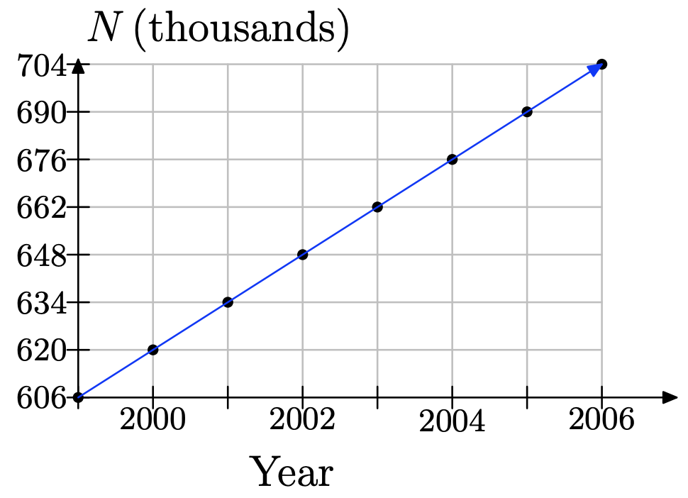
According to the Statistical Abstract of the United States (www.census.gov), there were approximately 606, 000 inmates in United States prisons in 1999, and this was increasing by a rate of about 14, 000 per year.
a) On a sheet of graph paper, make a coordinate system and plot the 1999 data as a point. Note that you will only need to graph the first quadrant of a coordinate system, since there are no data for years before 1999 and there cannot be a negative number of crimes reported. Use the given rate to find points for 2000 through 2006, and then draw a line through your data. We are constructing a continuous model for our discrete situation.
b) The following table lists the number of inmates, N, the year, and the number of years since 1999. In 1999, the number was 606, 000 and no occurrences of the 14, 000 increase had happened yet, so we fill in 606000 + 14000(0). In 2000, one occurrence of the 14, 000 increase had happened because one year had passed since 1999. Therefore, the number of crimes reported was 606000 + 14000(1). And the pattern continues in this manner. Fill in the remaining entries.
| Year | yrs x after ’99 | No. of inmates N |
|---|---|---|
| 1999 | 0 | 606000+14000(0) |
| 2000 | 1 | 606000+14000(1) |
| 2001 | ||
| 2002 |
c) Observing the pattern in the table, we come up with the equation N = 606000+14000x to relate the number of crimes C to the number of years x after 1999. Here, N is a function of x, and so we can use the notation N(x) = 606000+14000x to emphasis this.
i. Compute N(5).
ii. In a complete sentence, explain what N(5) represents.
iii. Compute N(7).
iv. In a complete sentence, explain what N(7) represents.
- Answer
-
a)
b)
Year yrs x after ’99 No. of inmates N 1999 0 606000+14000(0) 2000 1 606000+14000(1) 2001 2 606000+14000(2) 2002 3 606000+14000(3)
c)
i. N(5) = 606000 + 14000(5) = 676000.
ii. It means that, according to our model, 5 years after 1999 (that is, in 2004), the number of inmates will be 676, 000.
iii. N(7) = 606000 + 14000(7) = 704000.
iv. It means that, according to our model, in 2006, the number of inmates will be 704, 000
3.2 Exercises
Suppose you are riding a bicycle up a hill as shown below.

Figure \(\PageIndex{1}\). Riding a bicycle up a hill.
a) If the hill is straight as shown, consider the slant, or steepness, of its incline. As you ride up the hill, what can you say about the slant? Does it change? If so, how?
b) The slant is what mathematicians call the slope. To confirm your answer to part (a), you will place the hill on a coordinate system and compute its slope along various segments of the hill. See the figure below.
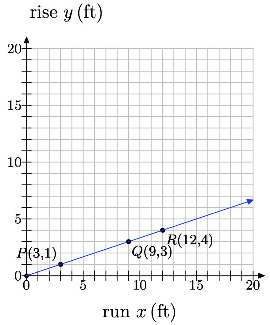
Three points–P, Q and R–have been labeled along the hill. We call the vertical distance (height) the rise and the horizontal distance the run. As you ride up the hill from point P to point Q, what is the rise? What is the run? Use these values to compute the slope from P to Q.
c) Now consider as you ride from P to R. What is the rise? What is the run? Use these values to compute the slope from P to R.
d) Finally, consider as you ride from Q to R. What is the rise? What is the run? Use these values to compute the slope from Q to R.
e) How do the values for slope from parts (b)-(d) compare? Do these results confirm your answer to part (a)?
f) Notice that the slope is positive in this example. In this context of riding a bicycle over a hill, what would negative slope mean?
- Answer
-
a) No, it does not change. The slant is the same everywhere along the straight hill.
b) \(m_{PQ} = \dfrac{3−1 }{9−3} = \dfrac{2}{6} = \dfrac{1}{3}\)
c) \(m_{PR} = \dfrac{4−1 }{12−3} = \dfrac{3}{9} = \dfrac{1}{3}\)
d) \(m_{QR} = \dfrac{4-3}{12−9} = \dfrac{1}{3}\)
e) They are all the same. This makes sense because the slant or steepness of the hill is the same throughout.
f) Positive slope means that you are riding uphill; negative slope would mean that you are riding downhill.
Set up a coordinate system on a sheet of graph paper, plotting the points P(3, 4) and Q(−2, −7) and drawing the line through them.
a) What can you say about the slope of the line? Is it positive, zero, negative or undefined? Is the slope the same everywhere along the line, or does it change in places? If it does change, where are the slopes different?
b) Use your graph to determine the change in y (rise) and the change in x (run). Use these results to compute the slope of the line.
c) Use the slope formula to compute the slope of the line.
d) Does your numerical solution from part (c) agree with your graphical solution from part (b)? If not, check your work for errors.
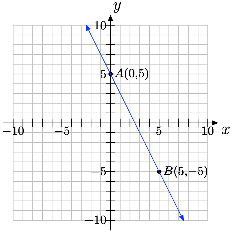
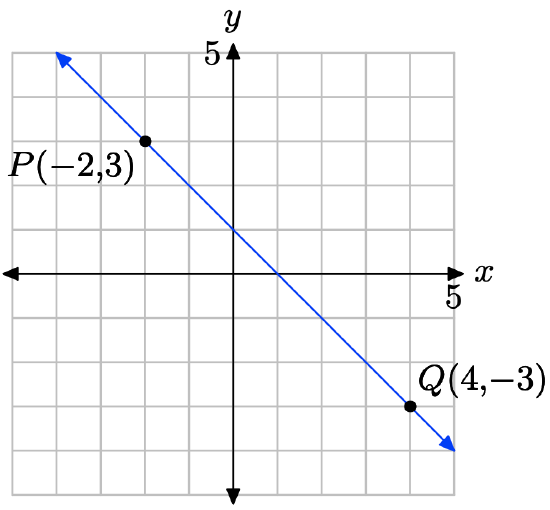
Set up a coordinate system on a sheet of graph paper, plotting the points P(−1, 3) and Q(5, −3) and drawing the line through them.
a) What can you say about the slope of the line? Is it positive, zero, negative or undefined? Is the slope the same everywhere along the line, or does it change in places? If it does change, where are the slopes different?
b) Use your graph to determine the change in y (rise) and the change in x (run). Use these results to compute the slope of the line.
c) Use the slope formula to compute the slope of the line.
d) Does your numerical solution from part (c) agree with your graphical solution from part (b)? If not, check your work for errors.
- Answer
-
a) The slope is negative because the line slants downhill. The slope is the same everywhere along the line because the slant of the line does not change.
b)
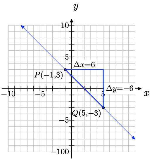
slope = −6/6 = −1
c) ∆y = −3 − (3) = −6; ∆x = 5 − (−1) = 6; slope = \dfrac{\delta y} {\delta x}\) =\( \dfrac{−6 }{6}\) = −1
d) Yes.
In Exercises \(\PageIndex{4}\)-\(\PageIndex{10}\), perform each of the following tasks.
i. Make a sketch of a coordinate system; plot the given points, and draw the line through the points.
ii. Use the slope formula to compute the slope of the line through the given points. Reduce the slope where possible.
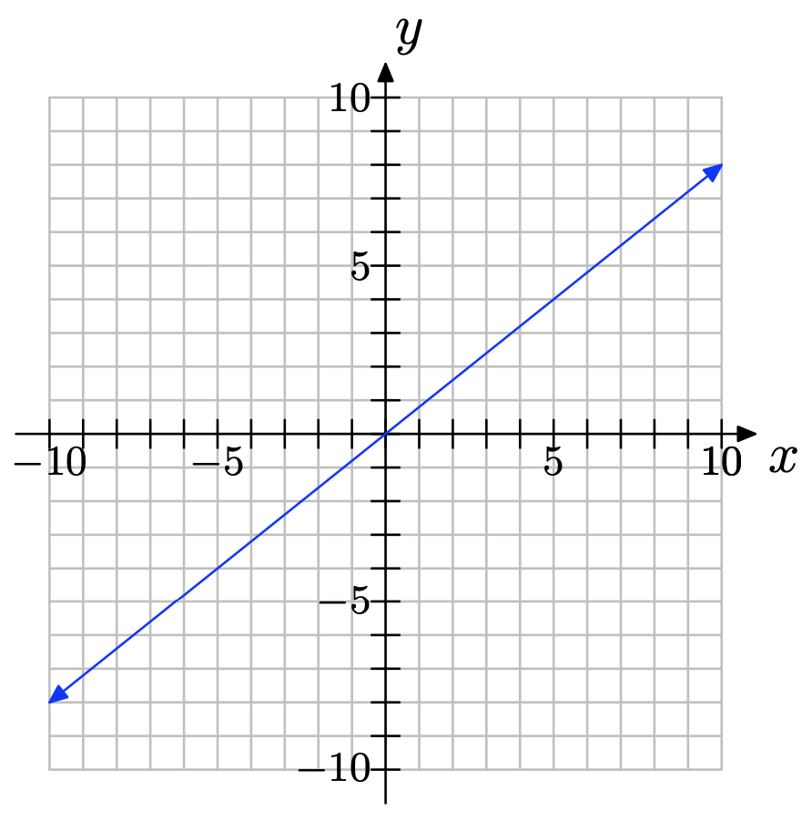
(0, 0) and (3, 4)
(−5, 2) and (0, 3)
- Answer
-
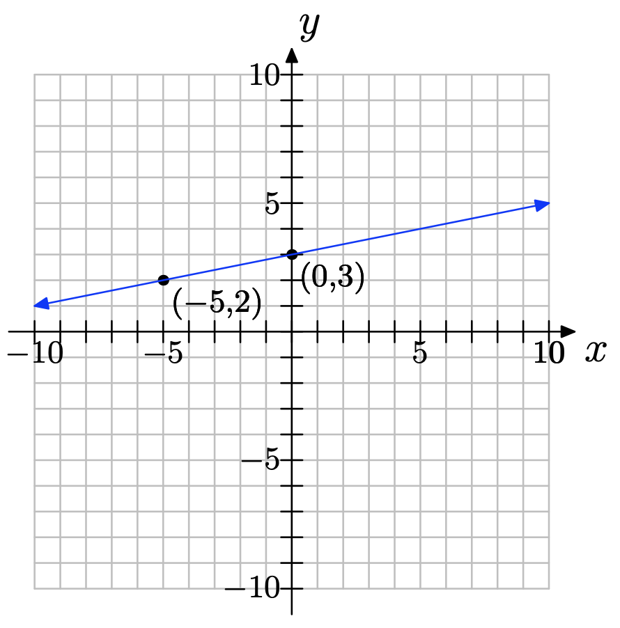
\(slope = \dfrac{3−2}{ 0−(−5)} = \dfrac{1}{5}\)
(−3, −3) and (6, −5)
(2, 0) and (2, 2)
- Answer
-
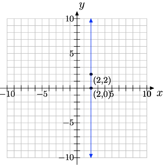
\(slope = \dfrac{2−0 }{2−2} = \dfrac{2}{0}\) = undefined
(−9, −3) and (6, −3)
(−8, 4) and (3, −8)
- Answer
-
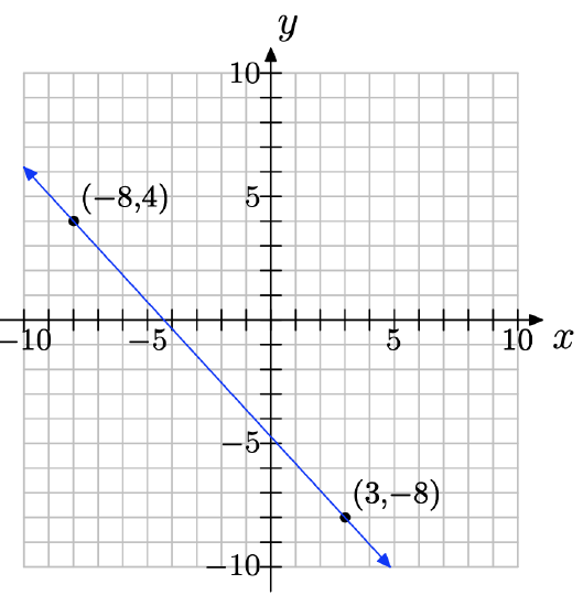
\(slope = \dfrac{−8−4}{ 3−(−8)} = \dfrac{−12}{ 11}\)
(−2, 6) and (5, −2)
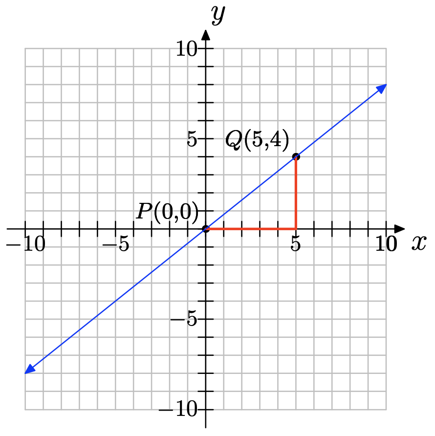
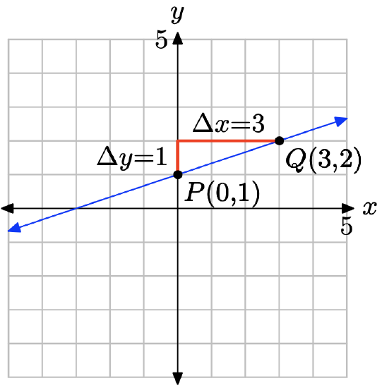
For the following line, two convenient points P and Q have been chosen. We chose two points that were at the corners of boxes on our grid so their coordinates are easy to read.
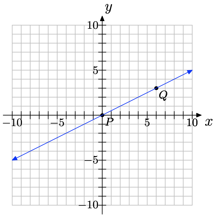
a) Label their coordinates.
b) Thinking of P as the starting point and Q as the ending point, draw a right triangle joining the points.
c) Clearly state the change in y (rise) and the change in x (run) from P to Q.
d) Compute the slope.
- Answer
-
a) The points are (0, 0) and (6, 3).
b)
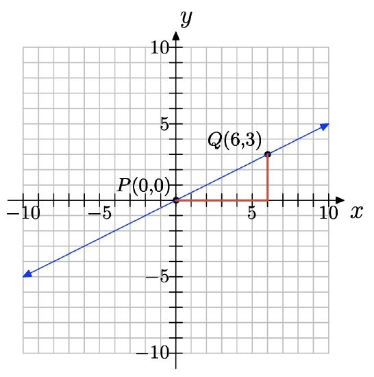
c) ∆y = 3 − 0 = 3; ∆x = 6 − 0 = 6
d) slope = \(\dfrac{\delta y}{\delta x} =\dfrac{3}{6} = \dfrac{1}{ 2}\)
For the following line, two convenient points A and B have been chosen. We chose two points that were at the corners of boxes on our grid so their coordinates are easy to read.
a) Label their coordinates.
b) Thinking of A as the starting point and B as the ending point, draw a right triangle joining the points.
c) Clearly state the change in y (rise) and the change in x (run) from A to B.
d) Compute the slope.
Copy the coordinate system below onto a sheet of graph paper. Then do the following:
a) Select any two convenient points P and Q on the graph of the line. Label each point with its coordinates.
b) Clearly state the change in y (rise) and the change in x (run). Compute the slope of the line.
- Answer
-
NOTE: Solutions may vary depending on which two convenient points were chosen.
a) You can pick any two points on the line; for example, (0, 0) and (5, 4) as shown below.
b) ∆y = 4 − 0 = 4; ∆x = 5 − 0 = 5; slope = \(\dfrac{\delta y }{\delta x} = \dfrac{4}{5}\)
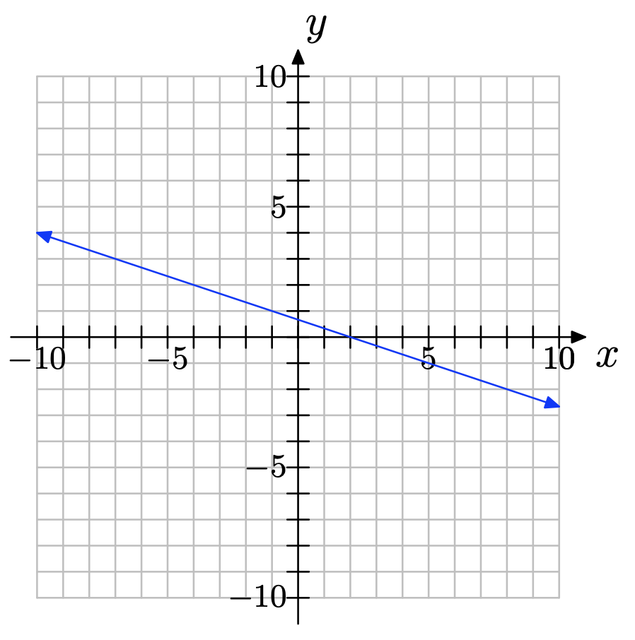
Copy the coordinate system below onto a sheet of graph paper. Then do the following:
a) Select any two convenient points P and Q on the graph of the line. Label each point with its coordinates.
b) Clearly state the change in y (rise) and the change in x (run). Compute the slope of the line.
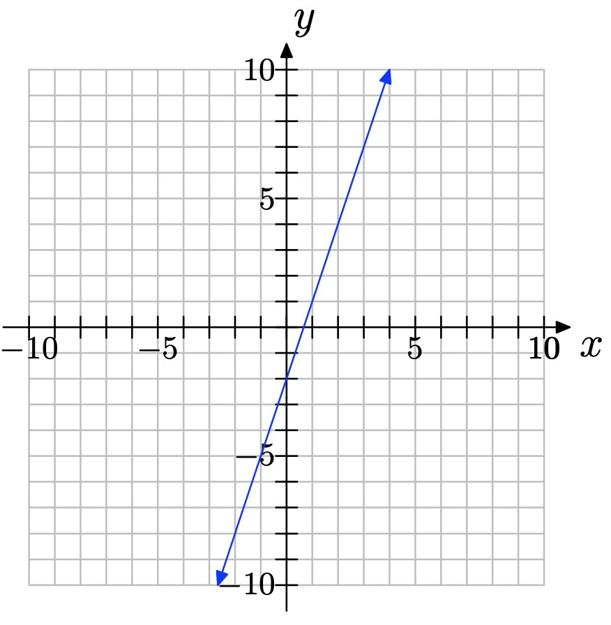
Copy the coordinate system below onto a sheet of graph paper. Then do the following:
a) Select any two convenient points P and Q on the graph of the line. Label each point with its coordinates.
b) Clearly state the change in y (rise) and the change in x (run). Compute the slope of the line.
- Answer
-
NOTE: Solutions may vary depending on which two convenient points were chosen.
a) You can pick any two points on the line; for example, (1, 1) and (3, 7) as shown below.
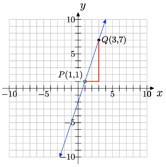
b) ∆y = 7 − 1 = 6; ∆x = 3 − 1 = 2; slope =\( \dfrac{\delta y }{\delta x} = \dfrac{6}{2} = 3\)
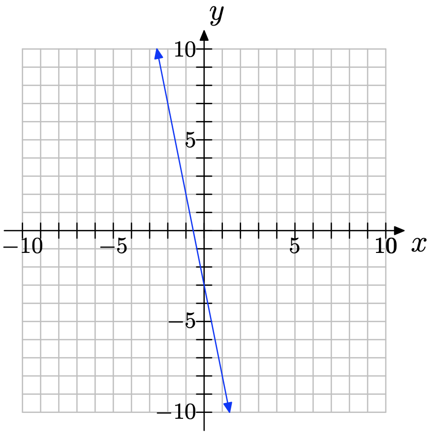
Copy the coordinate system below onto a sheet of graph paper. Then do the following:
a) Select any two convenient points P and Q on the graph of the line. Label each point with its coordinates.
b) Clearly state the change in y (rise) and the change in x (run). Compute the slope of the line.
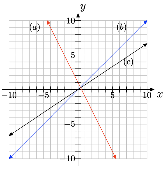
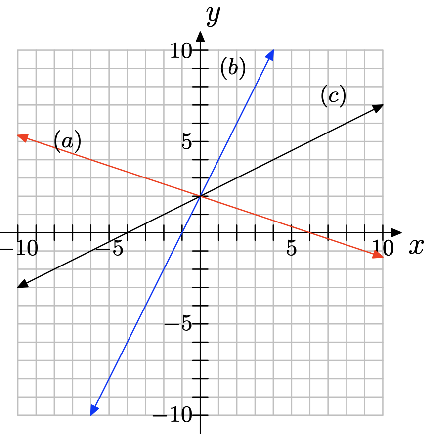
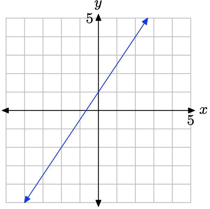
The following coordinate system shows the graphs of three lines, each with different slope. Match each slope with (a), (b), or (c) appropriately.
slope = 1
slope = 2/3
slope = −2
- Answer
-
slope = 1: (b)
slope = 2/3: (c)
slope = −2: (a)
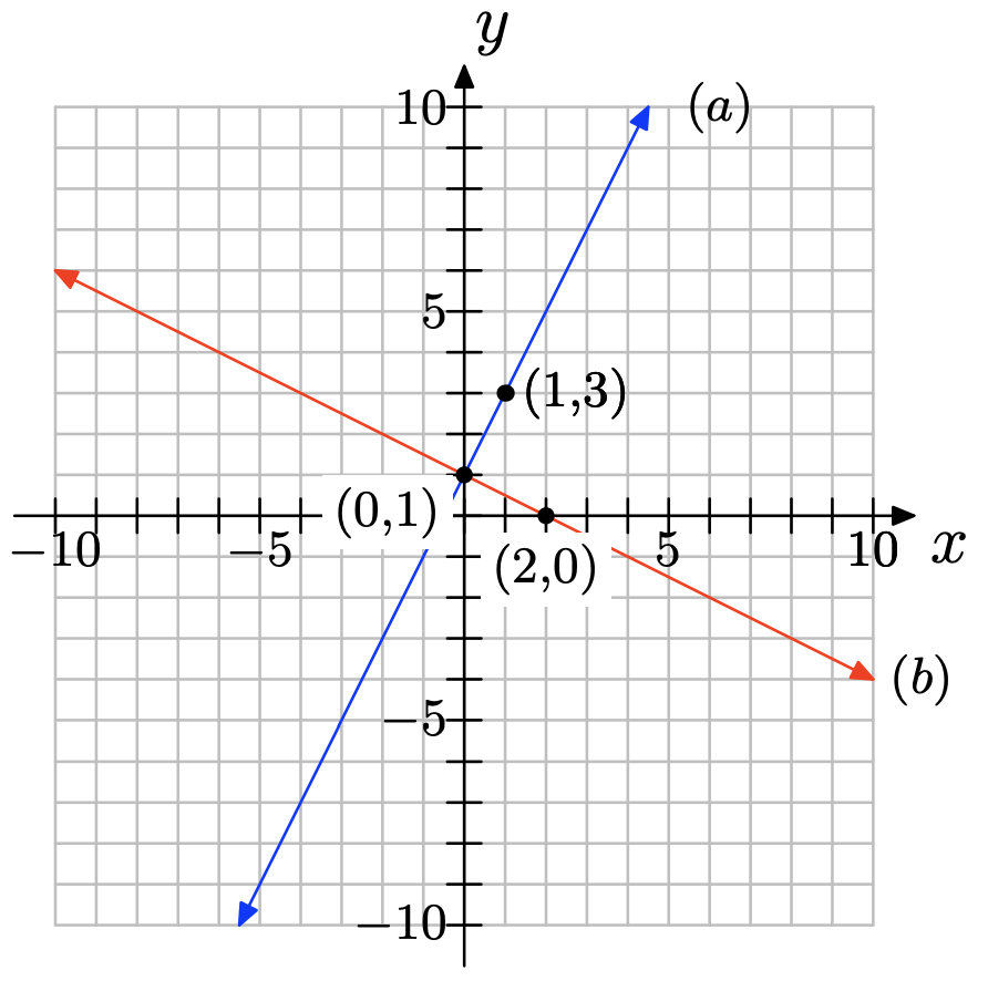
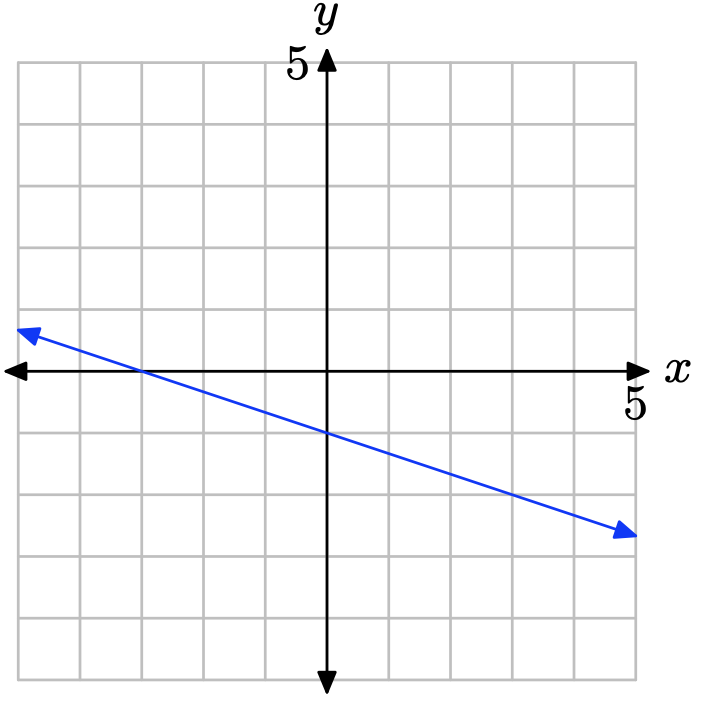
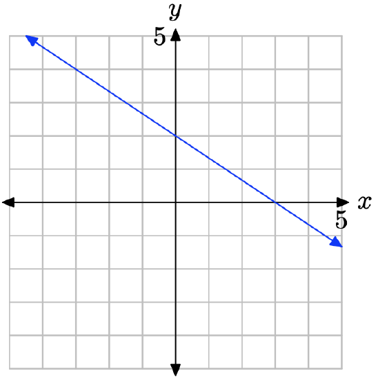
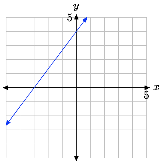
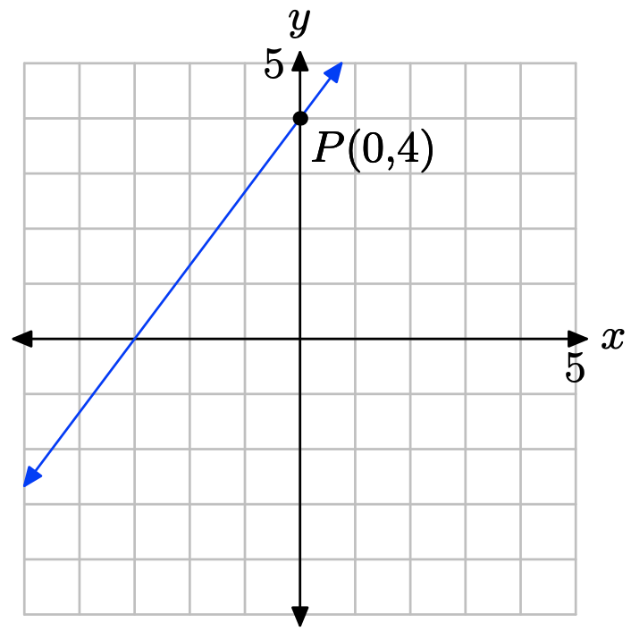
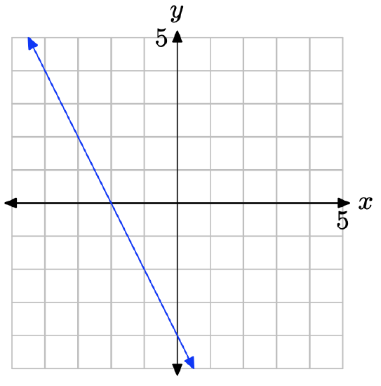
The following coordinate system shows the graphs of three lines, each with different slope. Match each slope with (a), (b), or (c) appropriately.
slope = 2
slope = −1/3
slope = 1/2
Draw a coordinate system on a sheet of graph paper for which the x- and y-axes both range from −10 to 10.
a) Draw a line that contains the point (0, 1) and has slope 2. Label the line as (a).
b) On the same coordinate system, draw a line that contains the point (0, 1) and has slope −1/2. Label it as (b).
c) Use the slopes of these two lines to show that they are perpendicular.
- Answer
-
b)
c) \(m_{1}m_{2} = 2(−1/2) = −1\), so the lines are perpendicular.
Draw a coordinate system on a sheet of graph paper for which the x- and y-axes both range from −10 to 10.
a) Draw a line that contains the point (1, −2) and has slope 1/3. Label the line as (a).
b) On the same coordinate system, draw a line that contains the point (0, 1) and has slope −3. Label it as (b).
c) Use the slopes of these two lines to show that they are perpendicular.
Draw a line through the point P(1, 3) that is parallel to the line through the origin with slope −1/4.
- Answer
-
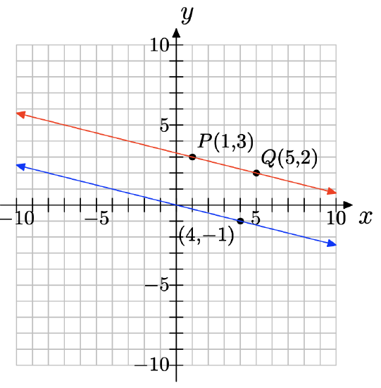
Draw a line through the point P(1,3) that is parallel to the line through the origin with slope 3/5.
Draw a coordinate system on a sheet of graph paper for which the x- and y-axes both range from −10 to 10.
a) Draw a line that contains the point (−1, −2) and has slope 3/4. Label the line as (a).
b) On the same coordinate system, draw a line that contains the point (0, 1) and has slope 4/3. Label it as (b).
c) Are these lines parallel, perpendicular or neither? Show using their slopes.
- Answer
-
b)
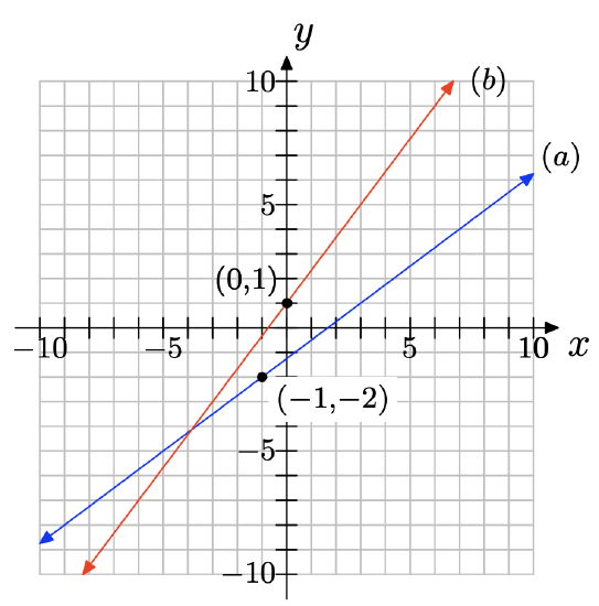
c) \(m_{1}m_{2} = (4/3)(3/4) = 1 \neq −1\), so the lines are not perpendicular; the slopes are not equal, so the lines are not parallel, either. Thus, the lines may be classified as neither parallel nor perpendicular.
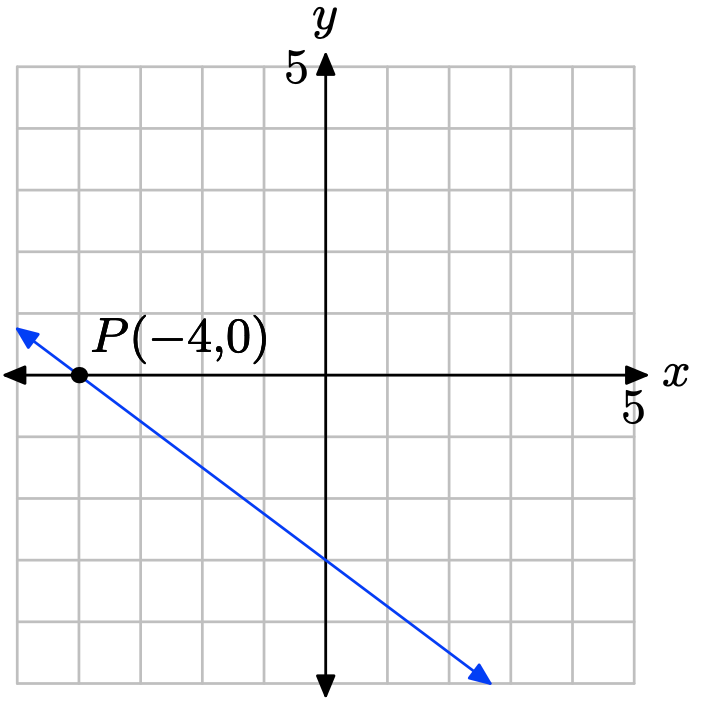
Graph a coordinate system on a sheet of graph paper for which the x- and y-axes both range from −10 to 10.
a) Draw a line that contains the point (−4, 0) and has slope 1. Label the line as (a).
b) On the same coordinate system, draw a line that contains the point (0, 2) and has slope −1. Label it as (b).
c) Are these lines parallel, perpendicular or neither? Show using their slopes.

Figure \(\PageIndex{2}\). A grade is a way of expressing slope.
On the road from Fort Bragg to Willits or from Fort Bragg to Santa Rosa, one often passes signs like that shown above. A grade is just slope expressed as a percent instead of a fraction or decimal. In other words, the grade measures the steepness of the road just as slope does.
a) An 80 /0 grade means that, for every horizontal distance of 100 ft, the road rises or drops 8 ft (depending on whether you are going uphill or downhill). Write 80 /0 grade as slope in reduced fractional form.
b) Suppose a hill drops 16 ft for every 180 ft horizontally. Find the grade of the hill to the nearest tenth of a percent.
c) Explain in a complete sentence or sentences what a grade of 00 /0 would represent.
- Answer
-
a) grade \(=\dfrac{ 8}{ 100} = \dfrac{2}{ 25}\)
b) grade \(= \dfrac{16}{ 180} = \dfrac{4}{ 45} = 8.90 \)%
c) 0% grade represents no grade or slope; that is, a flat road.
3.3 Exercises
In Exercises \(\PageIndex{1}\)-\(\PageIndex{6}\), perform each of the following tasks for the given linear function.
i. Set up a coordinate system on a sheet of graph paper. Label and scale each axis. Remember to draw all lines with a ruler.
ii. Identify the slope and y-intercept of the graph of the given linear function.
iii. Use the slope and y-intercept to draw the graph of the given linear function on your coordinate system. Label the y-intercept with its coordinate and the graph with its equation.
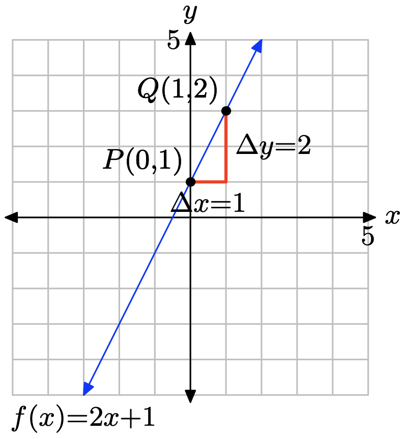
f(x) = 2x + 1
- Answer
-
Compare f(x) = 2x + 1 with f(x) = mx + b. Note that the slope is m = 2 and the y-coordinate of the y-intercept is b = 1. Therefore, the y-intercept will be the point (0, 1). Plot the point P(0, 1). To obtain a line of slope m = 2/1, start at the point P(0, 1), then move 1 unit to the right and 2 units upward, arriving at the point Q(1, 3), as shown in the figure below. The line through the points P and Q is the required line.
f(x) = −2x + 3
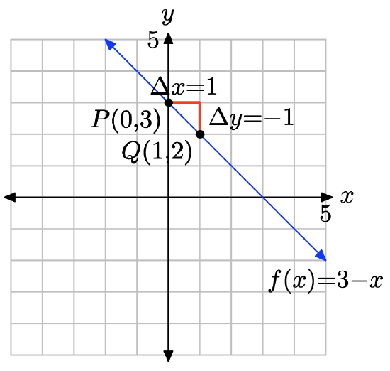
f(x) = 3 − x
- Answer
-
Compare f(x) = 3 − x, or equivalently f(x) = −x + 3, with f(x) = mx + b. Note that the slope is m = −1 and the y-coordinate of the y-intercept is b = 3. Therefore, the y-intercept will be the point (0, 3). Plot the point P(0, 3). To obtain a line of slope m = −1, start at the point P(0, 3), then move 1 unit to the right and 1 units downward, arriving at the point Q(1, 2), as shown in the figure below. The line through the points P and Q is the required line.
f(x) = 2 − 3x
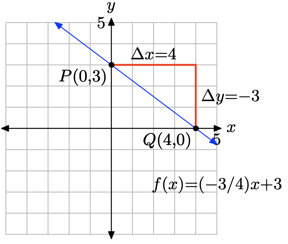
\(f(x) = −\frac{3}{4} x + 3\)
- Answer
-
Compare f(x) = (−3/4)x+3 with f(x) = mx+b. Note that the slope is m = −3/4 and the y-coordinate of the y-intercept is b = 3. Therefore, the y-intercept will be the point (0, 3). Plot the point P(0, 3). To obtain a line of slope m = −3/4, start at the point P(0, 3), then move 4 units to the right and 3 units downward, arriving at the point Q(4, 0), as shown in the figure below. The line through the points P and Q is the required line.
\(f(x) = \frac{2}{3} x − 2\)
In Exercises \(\PageIndex{7}\)-\(\PageIndex{12}\), perform each of the following tasks.
i. Make a copy of the given graph on a sheet of graph paper.
ii. Label the y-intercept with its coordinates, then draw a right triangle and label the sides to help identify the slope.
iii. Label the line with its equation.
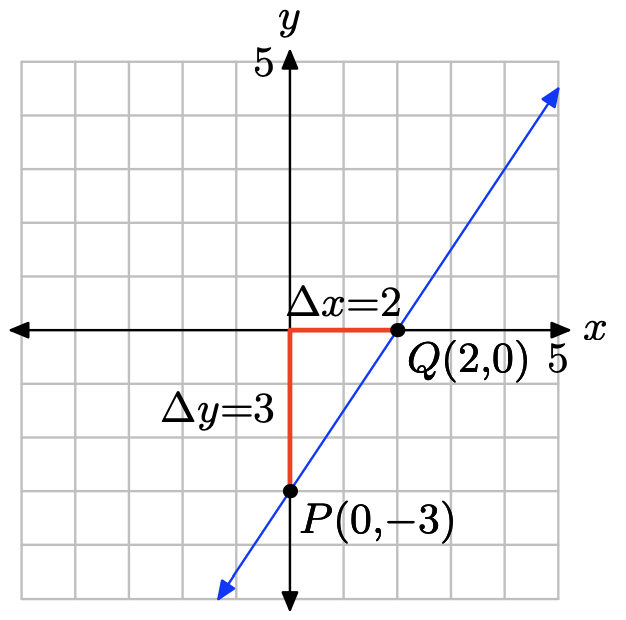
- Answer
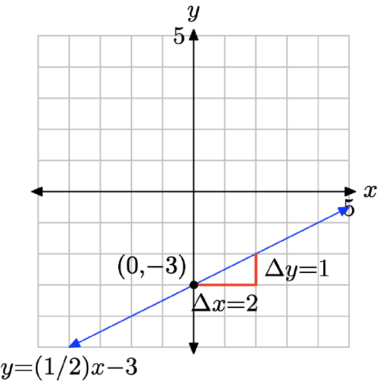
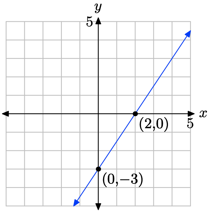
-
The slope is found by dividing the rise by the run (see figure). Hence, the slope is 1/2. The y-intercept is found by noting where the graph of the line crosses the y-axis (see figure), in this case, at (0, −3). Hence, m = 1/2 and b = −3, so the equation of the line in slope intercept form is
\[y = mx + b \quad \text{or} \quad y = \frac{1}{2}x − 3 \nonumber \]
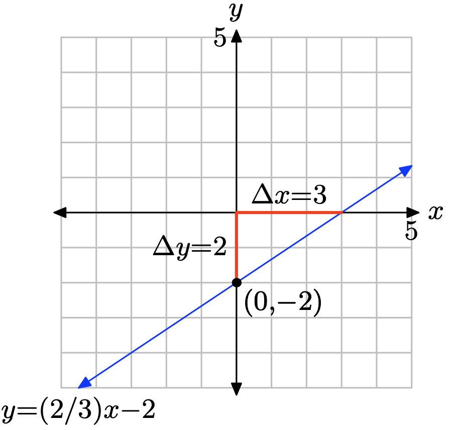
- Answer
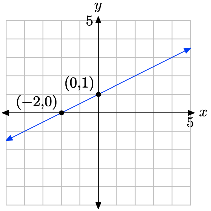
-
The slope is found by dividing the rise by the run (see figure). Hence, the slope is 2/3. The y-intercept is found by noting where the graph of the line crosses the y-axis (see figure), in this case, at (0, −2). Hence, m = 2/3 and b = −2, so the equation of the line in slope intercept form is
\[y = mx + b \quad \text{or} \quad y = \frac{2}{3}x − 2 \nonumber \]
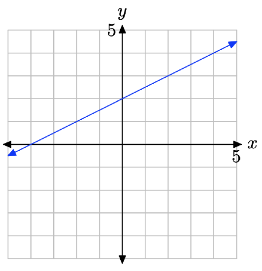
- Answer
-
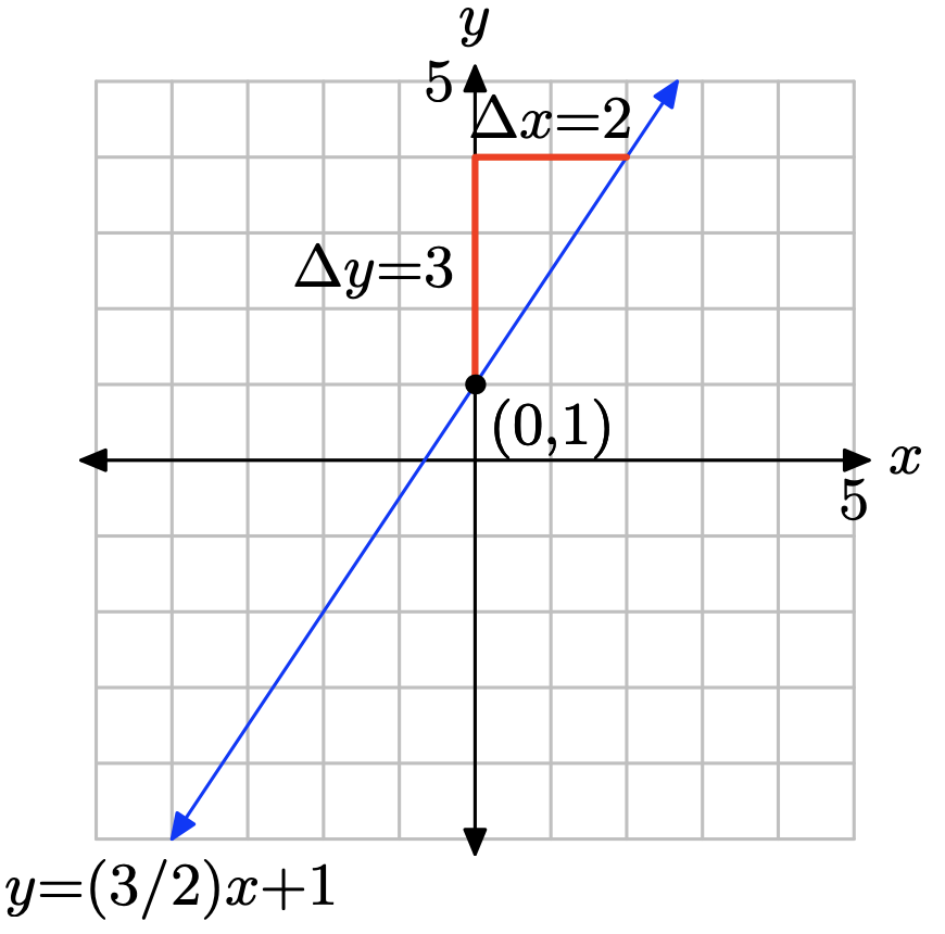
The slope is found by dividing the rise by the run (see figure). Hence, the slope is 3/2. The y-intercept is found by noting where the graph of the line crosses the y-axis (see figure), in this case, at (0, 1). Hence, m = 3/2 and b = 1, so the equation of the line in slope intercept form is
\[y = mx + b \quad \text{or} \quad y = \frac{3}{2}x + 1 \nonumber \]
Kate makes $39, 000 per year and gets a raise of $1000 each year. Since her salary depends on the year, let time t represent the year, with t = 0 being the present year, and place it along the horizontal axis. Let salary S, in thousands of dollars, be the dependent variable and place it along the vertical axis. We will assume that the rate of increase of $1000 per year is constant, so we can model this situation with a linear function.
a) On a sheet of graph paper, make a graph to model this situation, going as far as t = 10 years.
b) What is the S-intercept?
c) What is the slope?
d) Suppose we want to predict Kate’s salary in 20 years or 30 years. We cannot use the graphical model because it only shows up to t = 10 years. We could draw a larger graph, but what if we then wanted to predict 50 years into the future? The point is that a graphical model is limited to what it shows. A model algebraic function, however, can be used to predict for any year! Find the slope-intercept form of the linear function that models Kate’s salary.
e) Write the function using function notation, which emphasizes that S is a function of t.
f) Now use the algebraic model from (e) to predict Kate’s salary 10 years, 20 years, 30 years, and 50 years into the future.
g) Compute S(40).
h) In a complete sentence, explain what the value of S(40) from part (g) means in the context of the problem.
- Answer
-
a)
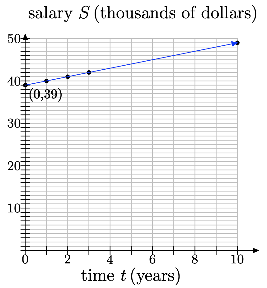
b) At t = 0 (present year), her salary is $39, 000. Since S is in thousands of dollars, S = 39 when t = 0. So the S-intercept is (0, 39).
c) The increase in Kate’s salary is $1, 000 per year, but S is in thousands of dollars, so the rate of increase in S is 1. That is, the slope is 1.
d) Using the slope-intercept form, we get S = t + 39.
e) S(t) = t + 39.
f)
- To find Kate’s salary in 10 years, compute S(10) = 10 + 39 = 49, which means that she will be earning $49, 000 per year.
- To find Kate’s salary in 20 years, compute S(20) = 20 + 39 = 59, which means that she will be earning $59, 000 per year.
- To find Kate’s salary in 30 years, compute S(30) = 30 + 39 = 69, which means that she will be earning $69, 000 per year.
- To find Kate’s salary in 50 years, compute S(50) = 50 + 39 = 89, which means that she will be earning $89, 000 per year.
g) S(40) = 40 + 39 = 79. h) If the current rate of increase continues, in 40 years Kate’s salary will be $79, 000.
For each DVD that Blue Charles Co. sells, they make 5c profit. Profit depends on the number of DVD’s sold, so let number sold n be the independent variable and profit P, in $, be the dependent variable.
a) On a sheet of graph paper, make a graph to model this situation, going as far as n = 15.
b) Use the graph to predict the profit if n = 10 DVD’s are sold.
c) The graphical model is limited to predicting for values of n on your graph. Any larger value of n necessitates a larger graph, or a different kind of model. To begin finding an algebraic model, identify the P-intercept of the graph.
d) What is the slope of the line in your graphical model?
e) Find a slope-intercept form of a linear function that models Blue Charles Co.’s sales.
f) Write the function using function notation.
g) Explain why this model does not have the same limitation as the graphical model.
h) Find P(100), P(1000), and P(10000).
i) In complete sentences, explain what the values of P(100), P(1000), and P(10000) mean in the context of the problem.
Enrique had $1, 000 saved when he began to put away an additional $25 each month.
a) Let t represent time, in months, and S represent Enrique’s savings, in $. Identify which should be the independent and dependent variables.
b) To begin finding a linear function to model this situation, identify the S-intercept and slope.
c) Find a slope-intercept form of a linear function to model Enrique’s savings over time.
d) Write the linear function in function notation.
e) Use the function model to predict how much will be in his savings in one year.
f) Use the function model to predict when will he have $2000 saved.
g) Graph the function on a coordinate system.
h) At the same time, Anne-Marie also begins to save $25 per month, but she begins with $1200 already in her savings. Make a graphical model of her situation and place it on the same coordinate system as the graphical model for Enrique’s savings. Label it appropriately.
i) How do the lines compare to each other? Say something about their slopes.
j) Find a slope-intercept form of a linear function that models Anne-Marie’s savings. Use the same variables as you did for Enrique’s model.
k) Write the function using function notation.
l) Prove that the graphs of the two functions are parallel lines.
m) For Anne-Marie, looking at the graphs, do you think it will take her more time or less time than Enrique to save up $2000?
n) Use the linear function model for Anne-Marie to predict how long it will take her to save $2000. Does this agree with your expectation from (m)?
- Answer
-
a) t should be the independent variable and S should be the dependent variable.
b) S-intercept = (0, 1000); slope = 25
c) S = 25t + 1000
d) S(t) = 25t + 1000
e) S(12) = 25(12) + 1000 = 1300
f) Set S=2000 and solve for t. 2000 = 25t + 1000 1000 = 25t 40 = t So it will take 40 months for him to reach $2000.
h)
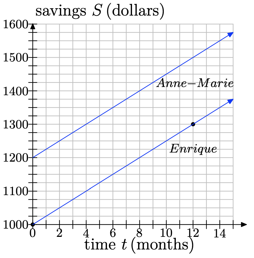
i) The lines have the same slope; they are parallel.
j) S = 25t + 1200
k) S(t) = 25t + 1200
l) They are lines because they are in the y = mx + b form. They are parallel because their slopes are equal (both are 25).
m) It should take her less time because her graph is above Enrique’s graph. This makes sense intuitively since she began with more money than he did.
n) Set S=2000 and solve for t. 2000 = 25t + 1200 800 = 25t 32 = t So it will take 32 months for her to reach $2000. This agrees with our expectation from (m): It takes her less time than Enrique
Jose is initially 400 meters away from the bus stop. He starts running toward the stop at a rate of 5 meters per second.
a) Express Jose’s distance d from the bus stop as a function of time t.
b) Use your model to determine Jose’s distance from the bus stop after one minute.
c) Use your model to determine the time it will take Jose to reach the bus stop.
A ball is dropped from rest above the surface of the earth. As it falls, its speed increases at a constant rate of 32 feet per second per second.
a) Express the speed v of the ball as a function of time t.
b) Use your model to determine the speed of the ball after 5 seconds.
c) Use your model to determine the time it will take for the ball to achieve a speed of 256 feet per second.
- Answer
-
a) We will do a “rough” plot of speed v versus time t. Speed depends upon time, so we place the speed on the vertical axis and the time on the horizontal axis in the figure that follows. The intial speed is 0 ft/s, which give us the v-intercept at P(0, 0). The rate at which the speed is increasing (acceleration) is constant and will be the slope of the line; i.e., the slope of the line is m = 32 ft/s2 (32 feet per second per second).
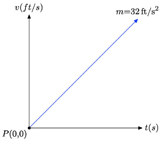
Because we know the slope and intercept of the line, we can use the slope intercept form y = mx + b and substitute m = 32 and b = 0 to obtain
\[y = mx + b\\ y = 32x + 0 \\y = 32x \nonumber \]
However, we are using v and t in place of y and x, so we replace these in the last formula to obtain
\[v = 32t \nonumber \]
or using function notation,
\[v(t) = 32t \nonumber \]
b) To find the speed of the ball after 5 seconds, substitute t = 5 into the equation developed in the previous part.\[v(t) = 32t \\ v(5) = 32(5) \\ v(5) = 160 \nonumber \]
Hence, the speed of the ball after 5 seconds is 160 feet per second.
c) To find the time it takes the ball to reach 256 feet per second, we must find t so that v(t) = 256.
\[v(t) = 256\\ 32t = 256\\ t = 8 \nonumber \]
Thus, it takes 8 seconds for the ball to attain a speed of 256 feet per second.
A ball is thrown into the air with an initial speed of 200 meters per second. It immediately begins to lose speed at a rate of 9.5 meters per second per second.
a) Express the speed v of the ball as a function of time t.
b) Use your model to determine the speed of the ball after 5 seconds.
c) Use your model to determine the time it will take for the ball to achieve its maximum height.
In Exercises \(\PageIndex{19}\)-\(\PageIndex{24}\), a linear function is given in standard form Ax + By = C. In each case, solve the given equation for y, placing the equation in slope-intercept form. Use the slope and intercept to draw the graph of the equation on a sheet of graph paper.
3x − 2y = 6
- Answer
-
Place 3x − 2y = 6 in slope-intercept form. First subtract 3x from both sides of the equation, then divide both sides of the resulting equation by −2.
\[\begin{array} {lll} 3x − 2y & = &6 −2 \\ y &=& −3x + 6 \\ y &= &\frac{3}{2}x − 3 \end{array} \nonumber \]
Compare y = (3/2)x − 3 with y = mx + b to see that the slope is m = 3/2 and the y-coordinate of the y-intercept is b = −3. Therefore, the y-intercept will be the point (0, −3). Plot the point P(0, −3). To obtain a line of slope m = 3/2, start at the point P(0, −3), then move 3 units up and 2 units to the right, arriving at the point Q(2, 0), as shown in the figure below. The line through the points P and Q is the required line.
3x + 5y = 15
3x + 2y = 6
- Answer
-
Place 3x + 2y = 6 in slope-intercept form. First subtract 3x from both sides of the equation, then divide both sides of the resulting equation by 2.
\[\begin{array}{lll} 3x + 2y & =& 6 \\ 2y &=& −3x + 6 \\ y &=& −\frac{3}{2} x + 3 \end{array} \nonumber \]
Compare y = (−3/2)x + 3 with y = mx + b to see that the slope is m = −3/2 and the y-coordinate of the y-intercept is b = 3. Therefore, the y-intercept will be the point (0, 3). Plot the point P(0, 3). To obtain a line of slope m = −3/2, start at the point P(0, 3), then move 3 units downward and 2 units to the right, arriving at the point Q(2, 0), as shown in the figure below. The line through the points P and Q is the required line.
4x − y = 4
x − 3y = −3
- Answer
-
Place x − 3y = −3 in slope-intercept form. First subtract x from both sides of the equation, then divide both sides of the resulting equation by −3.
\[\begin{array} {lll} x − 3y &=& −3 \\ −3y &=& −x − 3 \\ y &=& \frac{1}{3} x + 1 \end{array} \nonumber \]
Compare y = (1/3)x + 1 with y = mx + b to see that the slope is m = 1/3 and the y-coordinate of the y-intercept is b = 1. Therefore, the y-intercept will be the point (0, 1). Plot the point P(0, 1). To obtain a line of slope m = 1/3, start at the point P(0, 1), then move 1 unit upward and 3 units to the right, arriving at the point Q(3, 2), as shown in the figure below. The line through the points P and Q is the required line.
x + 4y = −4
In Exercises \(\PageIndex{25}\)-\(\PageIndex{30}\), you are given a linear function in slope-intercept form. Place the linear function in standard form Ax+ By = C, where A, B, and C are integers and A > 0.
\(y = \frac{2}{3}x − 5\)
- Answer
-
Start with \[y =\frac{ 2}{ 3} x − 5 \nonumber \] and multiply both sides by 3 to clear the fractions.
\[3y = 2x − 15 \nonumber \]
Finally, subtract 3y from both sides of the equation, then add 15 to both sides of the equation to obtain \[15 = 2x − 3y \nonumber \], or equivalently, \[2x − 3y = 15 \nonumber \].
\(y = \frac{5}{6}x + 1\)
\(y = −\frac{4}{ 5} x + 3\)
- Answer
-
Start with \[y = −\frac{4}{5} x + 3 \nonumber \] and multiply both sides by 5 to clear the fractions. \[5y = −4x + 15 \nonumber \]
Finally, add 4x to both sides of the equation.
\[4x + 5y = 15 \nonumber \]
\(y = −\frac{3}{7} x + 2\)
\(y = −\frac{2}{5} x − 3\)
- Answer
-
Start with \[y = −\frac{2}{5} x − 3 \nonumber \] and multiply both sides by 5 to clear the fractions.
\[5y = −2x − 15 \nonumber \]
Finally, add 2x to both sides of the equation.
\[2x + 5y = −15 \nonumber \]
\(y = −\frac{1}{4}x + 2\)
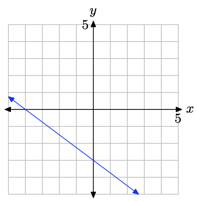
What is the x-intercept of the line?
- Answer
-
The x-intercept is the location where the line crosses the x-axis.
Therefore, the x-intercept is (−4, 0).
What is the y-intercept of the line?
What is the y-intercept of the line?
- Answer
-
The y-intercept is the location where the line crosses the y-axis.
Therefore, the y-intercept is (0, 4).
What is the x-intercept of the line?
In Exercises \(\PageIndex{35}\)-\(\PageIndex{40}\), find the x- and y-intercepts of the linear function that is given in standard form. Use the intercepts to plot the graph of the line on a sheet of graph paper.
3x − 2y = 6
- Answer
-
Set x = 0 in 3x − 2y = 6 to get −2y = 6 or y = −3. The y-intercept is (0, −3). Set y = 0 in 3x − 2y = 6 to get 3x = 6 or x = 2. The x-intercept is (2, 0). Plot the intercepts. The line through the intercepts is the required line.
4x + 5y = 20
x − 2y = −2
- Answer
-
Set x = 0 in x−2y = −2 to get −2y = −2 or y = 1. The y-intercept is (0, 1). Set y = 0 in x − 2y = −2 to get x = −2. The x-intercept is (−2, 0). Plot the intercepts. The line through the intercepts is the required line.
6x + 5y = 30
2x − y = 4
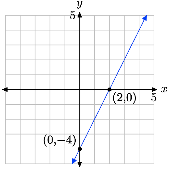
- Answer
-
Set x = 0 in 2x − y = 4 to get −y = 4 or y = −4. The y-intercept is (0, −4). Set y = 0 in 2x − y = 4 to get 2x = 4. The x-intercept is (2, 0). Plot the intercepts. The line through the intercepts is the required line.
8x − 3y = 24
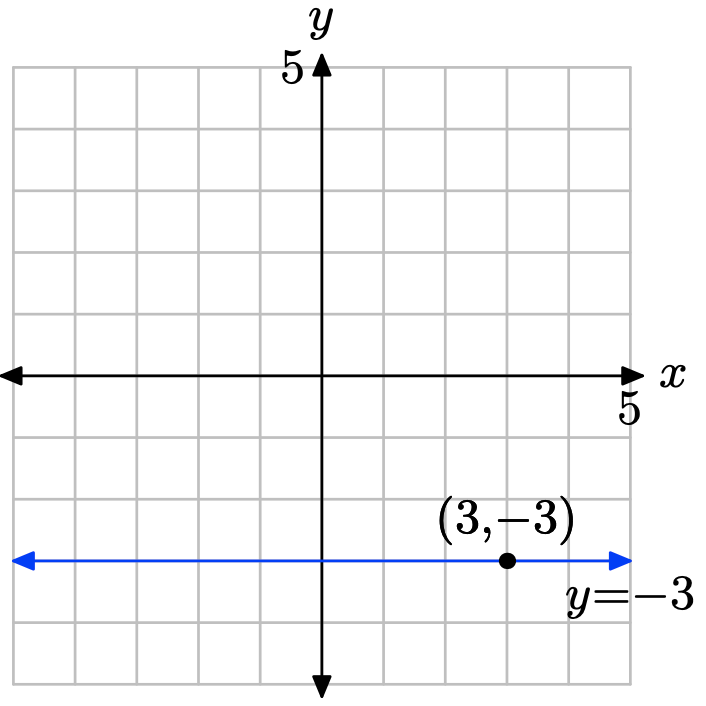
Sketch the graph of the horizontal line that passes through the point (3, −3). Label the line with its equation.
- Answer
-
Every horizontal line has an equation of the form y = d. Since this line must pass through the point (3, −3), it follows that the equation is y = −3.
Sketch the graph of the horizontal line that passes through the point (−9, 9). Label the line with its equation.
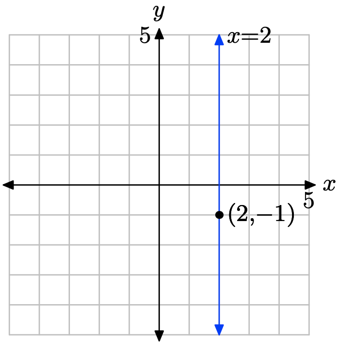
Sketch the graph of the vertical line that passes through the point (2, −1). Label the line with its equation.
- Answer
-
Every vertical line has an equation of the form x = c. Since this line must pass through the point (2, −1), it follows that the equation is x = 2.
Sketch the graph of the vertical line that passes through the point (15, −16). Label the line with its equation.
In Exercises \(\PageIndex{45}\)-\(\PageIndex{48}\), find the domain and range of the given linear function.
f(x) = −37x − 86
- Answer
-
The domain of every linear function is \((−\infty,\infty)\). Since the slope of the graph of f is \(−37 \neq 0\), the range is also \((−\infty,\infty)\).
f(x) = 98
f(x) = −12
- Answer
-
The domain of every linear function is \((−\infty,\infty)\). Since f(x) = −12 for every x, the range is {−12}.
f(x) = −2x + 8
3.4 Exercises
In Exercises \(\PageIndex{1}\)-\(\PageIndex{4}\), perform each of the following tasks.
i. Draw the line on a sheet of graph paper with the given slope m that passes through the given point \((x_{0}, y_{0})\).
ii. Estimate the y-intercept of the line.
iii. Use the point-slope form to determine the equation of the line. Place your answer in slope-intercept form by solving for y. Compare the exact value of the y-intercept with the approximation found in part (ii).
m = 2/3 and \((x_{0}, y_{0}) = (−1, −1)\)
- Answer
-
Plot the point P(−1, −1). To draw a line through P with slope m = 2/3, start at the point P, then move up 2 units and right 3 units to the point Q(2, 1). The line through the points P and Q is the required line.
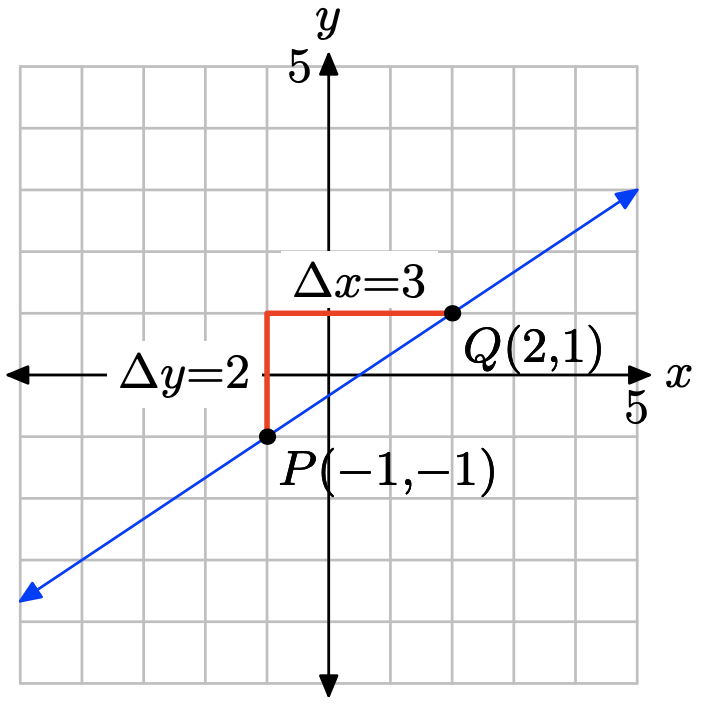
From the graph above, we would estimate the y-intercept as (0, −0.3). To find the equation of the line, substitute m = 2/3 and \((x_{0}, y_{0}) = (−1, −1)\) into the point-slope form of the line.
\[y − y0 = m(x − x0) \\ y − (−1) = \frac{2}{ 3} (x − (−1))\\ y + 1 = \frac{2}{ 3} (x + 1) \nonumber \]
To place this in slope-intercept form y = mx + b, solve for y.
\[y = \frac{2}{ 3} x + \frac{2}{ 3} − 1\\ y = \frac{2}{ 3} x + \frac{2}{ 3} − \frac{3}{ 3} \\ y = \frac{2}{ 3} x − \frac{1}{ 3} \nonumber \]
Comparing this result with y = mx + b, we see that the exact y-coordinate of the yintercept is b = −1/3, which is in close agreement with the approximation −0.3 found above.
m = -2/3 and \((x_{0}, y_{0}) = (1, −1)\)
m = -3/4 and \((x_{0}, y_{0}) = (−2, 3)\)
- Answer
-
Plot the point P(−2, 3). To draw a line through P with slope m = −3/4, start at the point P, then move down 3 units and right 4 units to the point Q(2, 0). The line through the points P and Q is the required line.
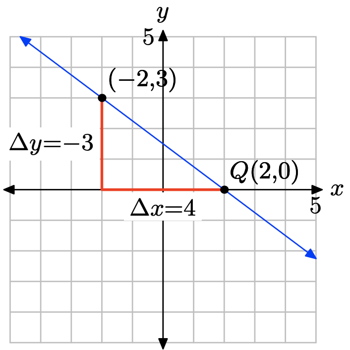
From the graph above, we would estimate the y-intercept as (0, 1.5). To find the equation of the line, substitute m = −3/4 and \((x_{0}, y_{0}) = (−2, 3)\) into the point-slope form of the line.
\[y − y_{0} = m(x − x_{0}) \\ y − 3 = −\frac{3}{ 4} (x − (−2)) \\ y − 3 = −\frac{3}{ 4} (x + 2) \nonumber \]
To place this in slope-intercept form y = mx + b, solve for y.
\[y = −\frac{3}{ 4} x − \frac{3}{ 2} + 3 \\ y = −\frac{3}{ 4} x − \frac{3}{ 2} + \frac{6}{ 2} \\ y = −\frac{3}{ 4} x + \frac{3}{ 2} \nonumber \]
Comparing this result with y = mx + b, we see that the exact y-coordinate of the y-intercept is b = 3/2, which is in close agreement with the approximation 1.5 found above.
m = 2/5 and \((x_{0}, y_{0}) = (−3, -2)\)
Find the equation of the line in slope-intercept form that passes through the point (1, 3) and has a slope of 1.
- Answer
-
Substitute 1 for m, 1 for \(x_{1}\), and 3 for \(y_{1}\) into the point-slope form \(y − y_{1} = m(x − x_{1})\) to obtain y − 3 = 1(x − 1). To place this in slope-intercept form y = mx + b, solve for y. \[y = x − 1 + 3 \\ y = x + 2 \nonumber \]
Find the equation of the line in slope-intercept form that passes through the point (0, 2) and has a slope of 1/4.
Find the equation of the line in slope-intercept form that passes through the point (1, 9) and has a slope of −2/3.
- Answer
-
Substitute −2/3 for m, 1 for x1, and 9 for y1 into the point-slope form \(y − y_{1} = m(x − x_{1})\)
to obtain \[y − 9 = −\frac{2}{3} (x − 1) \nonumber \].
To place this in slope-intercept form y = mx + b, solve for y.
\[y = −\frac{2}{3} x + \frac{2}{3} + 9 \\ y = −\frac{2}{3} x + \frac{2}{3} + \frac{27}{3} \\ y = −\frac{2}{3} x + \frac{29}{3} \nonumber \]
Find the equation of the line in slope-intercept form that passes through the point (1, 9) and has a slope of −3/4.
In Exercises \(\PageIndex{9}\)-\(\PageIndex{12}\), perform each of the following tasks.
i. Set up a coordinate system on a sheet of graph paper and draw the line through the two given points.
ii. Use the point-slope form to determine the equation of the line.
iii. Place the equation of the line in standard form Ax+By = C, where A, B, and C are integers and A > 0. Label the line in your plot with this result.
(−2, −1) and (3, 2)
- Answer
-
Plot the points P(−2, −1) and Q(3, 2) and draw a line through them.
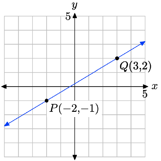
Calculate the slope of the line through the points P and Q.
\[m = \dfrac{\delta y }{\delta x} = \dfrac{2 − (−1)}{ 3 − (−2)} = \dfrac{3}{5} \nonumber \]
Substitute m = 3/5 and \((x_{0}, y_{0}) = (−2, −1)\) into the point-slope form of the line
\[y − y_{0} = m(x − x_{0}) \\ y − (−1) = \dfrac{3}{5} (x − (−2)) \\ y + 1 =\dfrac{3}{5} (x + 2) \nonumber \]
Place this result in Standard form. First clear the fractions by multiplying by 5.
\[y + 1 = \dfrac{3}{5} x + \dfrac{6}{5} \\ 5y + 5 = 3x + 6 \\ 3x − 5y = −1 \nonumber \]
Hence, the standard form of the line is 3x − 5y = −1.
(−1, 4) and (2, −3)
(−2, 3) and (4, −3)
- Answer
-
Plot the points P(−2, 3) and Q(4, −3) and draw a line through them.
Calculate the slope of the line through the points P and Q.
\[m = \dfrac{\delta y}{\delta x} = \dfrac{−3 − 3}{4 − (−2)}= \dfrac{−6}{ 6} = −1 \nonumber \]
Substitute m = −1 and \((x_{0}, y_{0}) = (−2, 3)\) into the point-slope form of the line.
\[y − y_{0} = m(x − x_{0}) \\ y − 3 = −1(x − (−2)) \\ y − 3 = −1(x + 2) \nonumber \]
Place this result in Standard form.
\[y − 3 = −x − 2 \\ x + y = 1 \nonumber \]
Hence, the standard form of the line is x + y = 1.
(−4, 4) and (2, −4)
Find the equation of the line in slope-intercept form that passes through the points (−5, 5) and (6, 8).
- Answer
-
Substitute 5 for \(y_{1}\), 8 for \(y_{2}\), −5 for \(x_{1}\), and 6 for \(x_{2}\) into the slope formula to find the slope m:
\[m = \dfrac{y_{1} − y_{2}}{x_{1} − x_{2} }= \dfrac{5 − 8}{−5 − 6} = \dfrac{3}{11} \nonumber \]
Now substitute \(\dfrac{3}{11}\) for m, −5 for x1, and 5 for y1 into the point-slope form
\[y − y_{1} = m(x − x_{1}) \nonumber \]
and then solve for y to obtain the equation
\[y = \dfrac{3}{ 11} x + \dfrac{70}{ 11} \nonumber \]
Find the equation of the line in slope-intercept form that passes through the points (6, −6) and (9, −7).
Find the equation of the line in slope-intercept form that passes through the points (−4, 6) and (2, −4).
- Answer
-
Substitute 6 for \(y_{1}\), −4 for \(y_{2}\), −4 for \(x_{1}\), and 2 for \(x_{2}\) into the slope formula to find the slope m:
\[m = \dfrac{ y_{1} − y_{2}}{ x_{1} − x_{2} }= \dfrac{6 − (−4) }{−4 − 2} = \dfrac{−5}{ 3} \nonumber \]
Now substitute \(\dfrac{−5}{ 3}\) for m, −4 for x1, and 6 for \(y_{1}\) into the point-slope form
\[y − y_{1} = m(x − x_{1}) \nonumber \]
and then solve for y to obtain the equation
\[y = \dfrac{−5}{3} x − \dfrac{2}{ 3} \nonumber \]
Find the equation of the line in slope-intercept form that passes through the points (−1, 5) and (4, 4).
In Exercises \(\PageIndex{17}\)-\(\PageIndex{20}\), perform each of the following tasks.
i. Draw the graph of the given linear equation on graph paper and label it with its equation.
ii. Determine the slope of the given equation, then use this slope to draw a second line through the given point P that is parallel to the first line.
iii. Estimate the y-intercept of the second line from your graph.
iv. Use the point-slope form to determine the equation of the second line. Place this result in slope-intercept form y = mx + b, then state the exact value of the y-intercept. Label the second line with the slope-intercept form of its equation.
2x + 3y = 6, P = (−2, −3)
- Answer
-
Plot the points Q(0, 2) and R(3, 0) and draw a line through them as shown in (a) below. You can calculate the slope of this line from the graph, or you can use the slope formula as follows.
\[m = \dfrac{\delta y}{\delta x} = \dfrac{0 − 2 }{3 − 0} = −\dfrac{2}{ 3} \nonumber \]
The second line must be parallel to the first, so it must have the same slope; namely, m = −2/3. The second line must pass through the point P(−2, −3), so plot the point P. To get the right slope, start at the point P, then move 3 units to the right and 2 units down, as shown in (b). It would appear that this line crosses the y-axis near (0, −4.3).
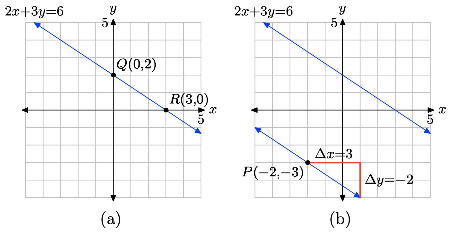
To find the equation of the second line, use the point slope form of the line and m = −2/3 and \((x_{0}, y_{0}) = (−2, −3)\), as follows.
\[y − y_{0} = m(x − x_{0}) \\ y − (−3) = −\dfrac{2}{ 3} (x − (−2)) \\ y + 3 = −\dfrac{2}{ 3}(x + 2) \nonumber \]
To place this in slope-intercept form y = mx + b, we must solve for y.
\[y + 3 = −\dfrac{2}{ 3}x − \dfrac{4}{ 3} \\ y = −\dfrac{2}{ 3} x − \dfrac{4}{ 3} − 3 \\ y = −\dfrac{2}{ 3} x − \dfrac{4}{ 3} −\dfrac{9}{ 3}\\ y = −\dfrac{2}{ 3} x − \dfrac{13}{ 3} \nonumber \]
Hence, the equation in slope-intercept form is y = (−2/3)x − 13/3, making the exact y-coordinate of the y-intercept b = −13/3, which is in pretty close agreement (check on your calculator) with our estimate of −4.3.
3x − 4y = 12, P = (−3, 4)
x + 2y = −4, P = (3, 3)
- Answer
-
Plot the points Q(−4, 0) and R(0, −2) and draw a line through them as shown in (a) below. You can calculate the slope of this line from the graph, or you can use the slope formula as follows.
\[m = \dfrac{\delta y}{\delta x} = \dfrac{−2 − 0 }{0 − (−4)} = −\dfrac{1}{2} \nonumber \]
The second line must be parallel to the first, so it must have the same slope; namely, m = −1/2. The second line must pass through the point P(3, 3), so plot the point P. To get the right slope, start at the point P, then move 1 unit downward and 2 units to the right, as shown in (b). It would appear that this line crosses the y-axis near (0, 4.5).
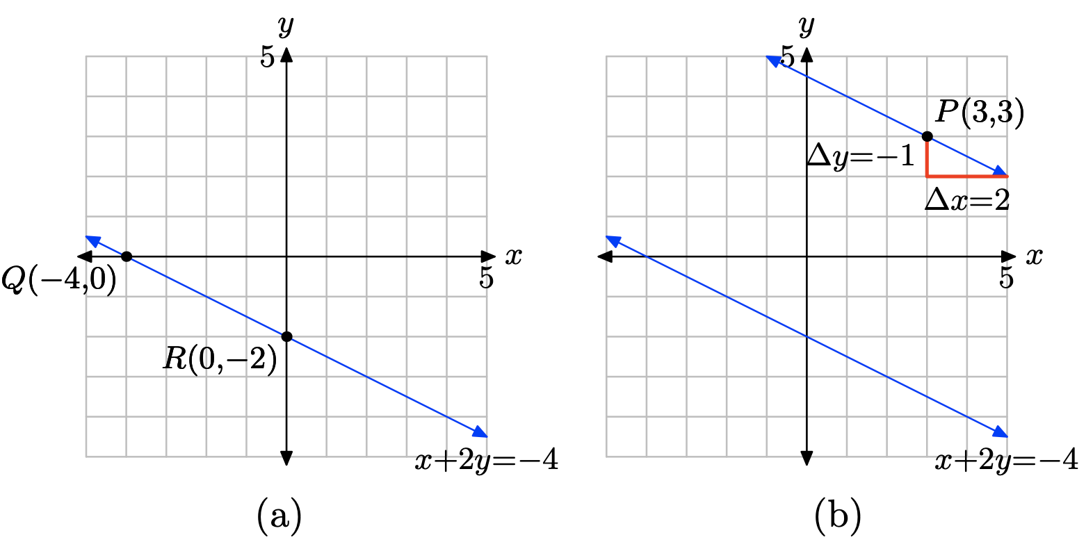
To find the equation of the second line, use the point slope form of the line and m = −1/2 and \((x_{0}, y_{0}) = (3, 3)\), as follows.
\[y − y_{0} = m(x − x_{0}) \\ y − 3 = −\dfrac{1}{ 2} (x − 3) \nonumber \]
To place this in slope-intercept form y = mx + b, we must solve for y.
\[− 3 = −\dfrac{1}{ 2} x + \dfrac{3}{ 2} \\ y = −\dfrac{1}{ 2} x + \dfrac{3}{ 2} + 3 \\ y = −\dfrac{1}{ 2} x + \dfrac{3}{ 2} + \dfrac{6}{ 2} \\ y = −\dfrac{1}{ 2} x + \dfrac{9}{ 2} \nonumber \]
Hence, the equation in slope-intercept form is y = (−1/2)x + 9/2, making the exact y-coordinate of the y-intercept b = 9/2, which is in pretty close agreement (check on your calculator) with our estimate of 4.5.
5x + 2y = 10, P = (−3, −5)
In Exercises \(\PageIndex{21}\)-\(\PageIndex{24}\), perform each of the following tasks.
i. Draw the graph of the given linear equation on graph paper and label it with its equation.
ii. Determine the slope of the given equation, then use this slope to draw a second line through the given point P that is prependicular to the first line.
iii. Use the point-slope form to determine the equation of the second line. Place this result in standard form Ax+By = C, where A, B, C are integers and A > 0. Label the second line with this standard form of its equation.
x − 2y = −2, P = (3, −4)
- Answer
-
Let x = 0 in x − 2y = −2. Then −2y = −2 and y = 1. This calculation gives us the y-intercept R(0, 1). Let y = 0 in x − 2y = −2 and x = −2. This gives us the x-intercept Q(−2, 0). Plot the points Q(−2, 0) and R(0, 1) and draw a line through them as in (a) below.
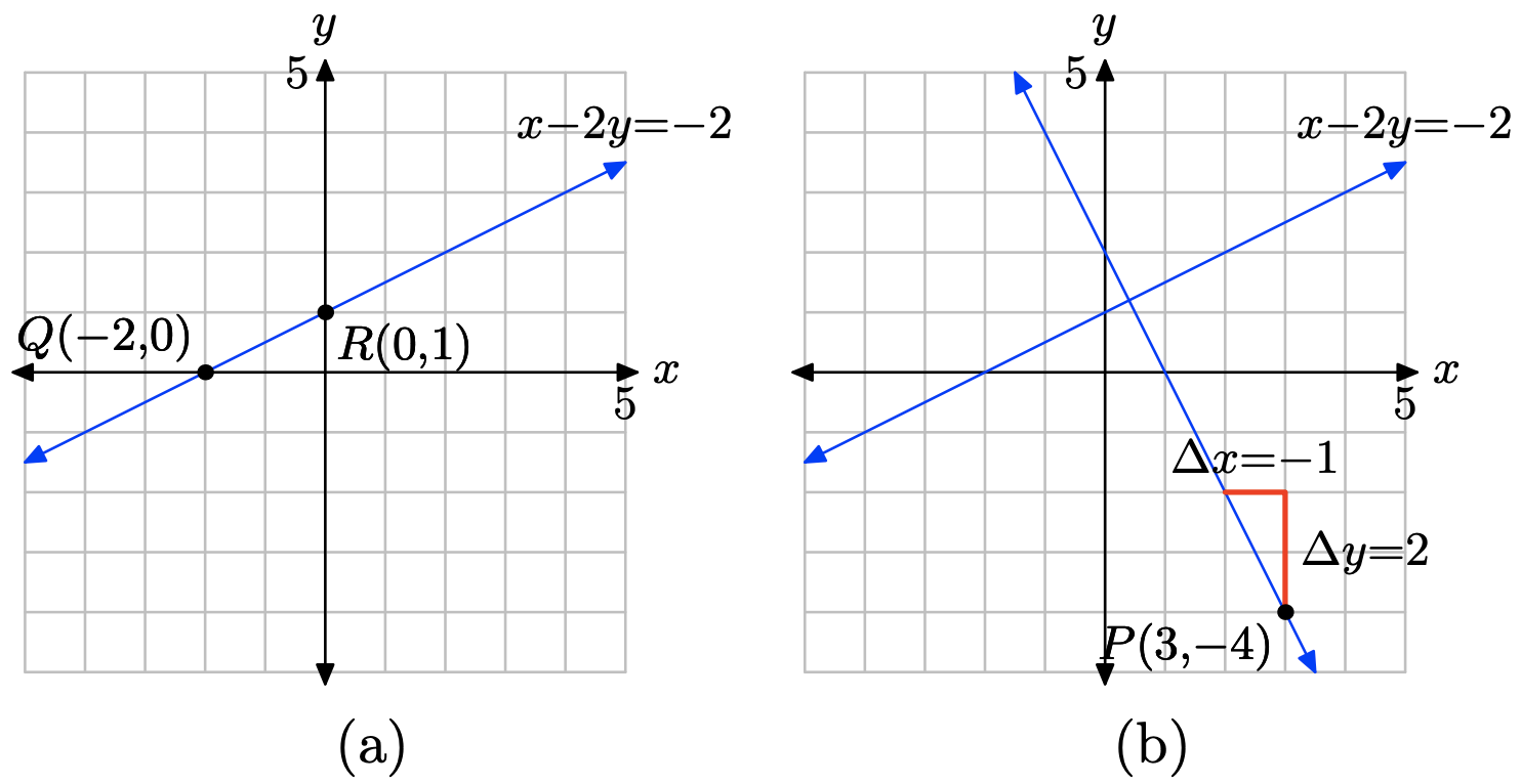
You can calculate the slope of the first line from the graph or you can obtain it with the slope formula as follows.
\[m1 = \dfrac{\delta y}{\delta x} = \dfrac{1 − 0}{ 0 − (−2)} = \dfrac{1}{ 2} \nonumber \]
The second line is perpendicular to this first line, so the slope of the second line must be the negative reciprocal of the slope of the first line; i.e., the slope of the second line should be \(m = −1/m_{2} = −1/(1/2)\), or m = −2. To draw a line through the point P(3, −4) that is perpendicular to the line in (a), first plot the point P(3, −4), then move upward 2 units and to the left 1 unit as shown in (b). This gives us a line through P(3, −4) with slope m = −2, so this line will be perpendicular to the first line. To find the equation of the perpendicular line, substitute m = −2 and \((x_{0}, y_{0}) = (3, −4)\) into the point-slope formula, then place the resulting equation in standard form.
\[y − y_{0} = m(x − x_{0}) \\ y − (−4) = −2(x − 3) \\ y + 4 = −2x + 6 \\ 2x + y = 2 \nonumber \]
Thus, the equation of the line that passes through P(3, −4) and is perpendicular to the line x − 2y = −2 is 2x + y = 2.
3x + y = 3, P = (−3, −4)
x − 2y = 4, P = (−3, 3)
- Answer
-
Set x = 0 in x − 2y = 4 to obtain −2y = 4. Hence, y = −2 and the y-intercept is Q(0, −2). Set y = 0 in x − 2y = 4 to obtain x = 4. Hence, the x-intercept is R(4, 0). Plot Q(0, −2) and R(4, 0) and draw a line through them as in (a) below.
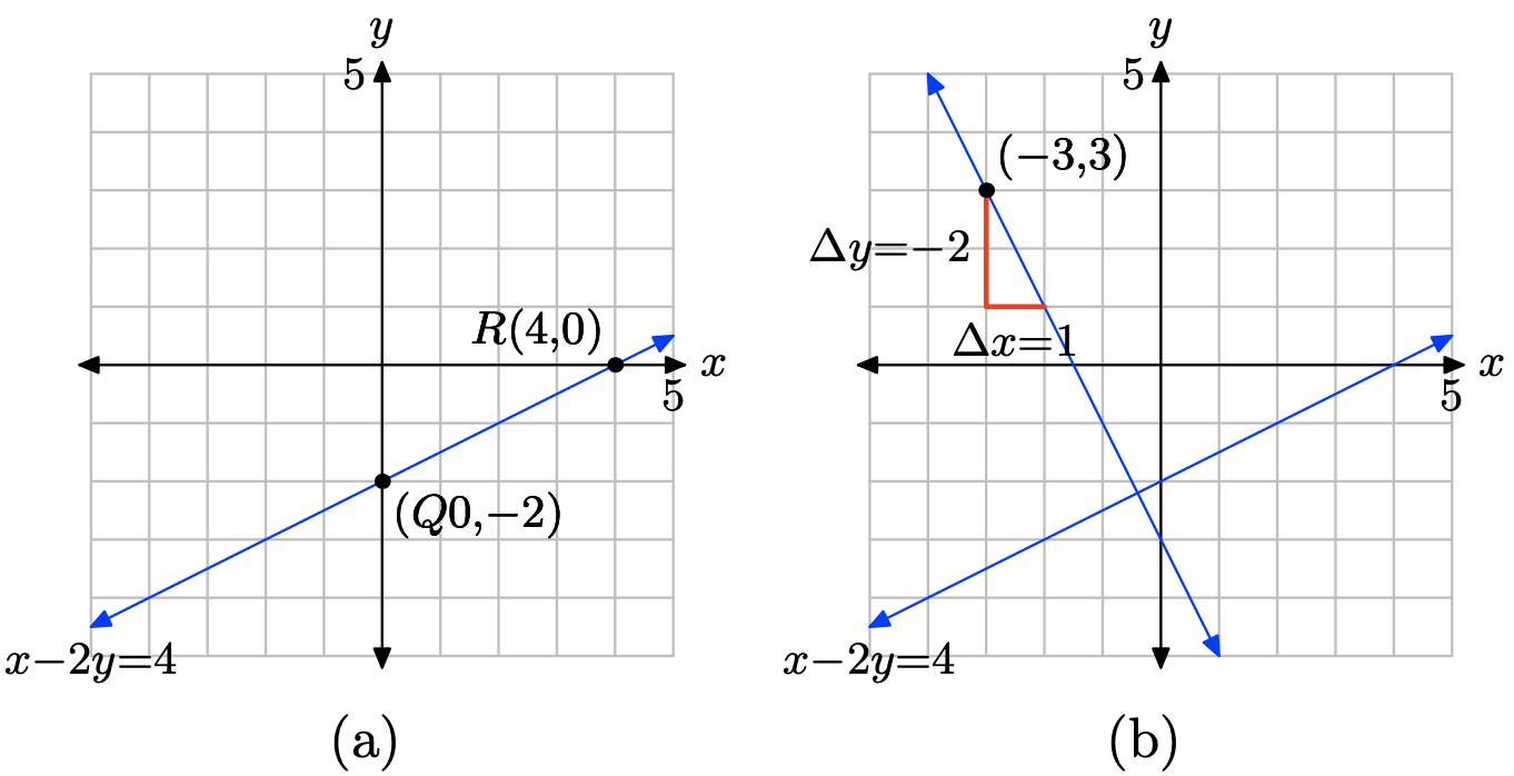
You can calculate the slope of the first line from the graph or you can obtain it with the slope formula as follows.
\[m_{1} = \dfrac{\delta y}{\delta x} = \dfrac{0 − (−2)}{ 4 − 0 }= \dfrac{1}{2} \nonumber \]
The second line is perpendicular to this first line, so the slope of the second line must be the negative reciprocal of the slope of the first line; i.e., the slope of the second line should be m = −1/m2 = −1/(1/2), or m = −2. To draw a line through the point P(−3, 3) that is perpendicular to the line in (a), first plot the point P(−3, 3), then move downward 2 units and to the right 1 unit as shown in (b). This gives us a line through P(−3, 3) with slope m = −2, so this line will be perpendicular to the first line. To find the equation of the perpendicular line, substitute m = −2 and \((x_{0}, y_{0}) = (−3, 3)\) into the point-slope formula, then place the resulting equation in standard form.
\[y − y_{0} = m(x − x_{0}) \\ y − 3 = −2(x − (−3)) \\ y − 3 = −2(x + 3) \\ y − 3 = −2x − 6 \\ 2x + y = −3 \nonumber \]
Thus, the equation of the line that passes through P(−3, 3) and is perpendicular to the line x − 2y = 4 is 2x + y = −3.
x − 4y = 4, P = (−3, 4)
Find the equation of the line in slope-intercept form that passes through the point (7, 8) and is parallel to the line x − 5y = 4.
- Answer
-
First solve x − 5y = 4 for y to get \(y = \dfrac{1 }{5} x − \dfrac{4}{5} \) The slope of this line is \(\dfrac{1}{5}\). Therefore, every parallel line also has slope \(\dfrac{1}{5}\).
Now to find the equation of the parallel line that passes through the point (7, 8), substitute \(\dfrac{1}{5}\) for m, 7 for \(x_{1}\), and 8 for \(y_{1}\) into the point-slope form
\[y − y_{1} = m(x − x_{1}) \nonumber \] to obtain
\[y − 8 = \dfrac{1}{5}(x − 7) \nonumber \]. Then solve for y:
\[y = \dfrac{1}{5} x − \dfrac{7}{5} + 8 \\ y = \dfrac{1}{5}x − \dfrac{7}{5} +\dfrac{40}{5} y = \dfrac{1}{5} x + \dfrac{33}{5} \nonumber \]
Find the equation of the line in slope-intercept form that passes through the point (3, −7) and is perpendicular to the line 7x − 2y = −8.
Find the equation of the line in slope-intercept form that passes through the point (1, −2) and is perpendicular to the line −7x + 5y = 4.
- Answer
-
First solve −7x + 5y = 4 for y to get
\[y = \dfrac{7}{5} x + 4 5 \nonumber \]
The slope of this line is \dfrac{7}{5}. Therefore, every perpendicular line has slope −\(\dfrac{7}{5}\) (the negative reciprocal of \(\dfrac{7}{5}\). Now to find the equation of the perpendicular line that passes through the point (1, −2), substitute −\dfrac{5}{7} for m, 1 for \(x_{1}\), and −2 for \(y_{1}\) into the point-slope form
\[y − y1 = m(x − x1) \nonumber \] to obtain \[y − (−2) = −\dfrac{5}{7} (x − 1) \nonumber \]. Then solve for y:
\[y = −\dfrac{5}{7}x +\dfrac{5}{7} − 2 \\ y = −\dfrac{5}{7} x + \dfrac{5}{7} − \dfrac{14}{7} \\ y = −\dfrac{5}{7} x − \dfrac{9}{7} \nonumber \]
Find the equation of the line in slope-intercept form that passes through the point (4, −9) and is parallel to the line 9x + 3y = 5.
Find the equation of the line in slope-intercept form that passes through the point (2, −9) and is perpendicular to the line −8x + 3y = 1.
- Answer
-
First solve −8x + 3y = 1 for y to get \[y = \dfrac{8}{3} x + \dfrac{1}{3} \nonumber \]
The slope of this line is \(\dfrac{8}{3}\). Therefore, every perpendicular line has slope \(−\dfrac{3}{8}\) (the negative reciprocal of \(\dfrac{8}{3}\)). Now to find the equation of the perpendicular line that passes through the point (2, −9), substitute \(−\dfrac{3}{8}\) for m, 2 for \(x_{1}\), and −9 for \(y_{1}\) into the point-slope form \[y − y1 = m(x − x1) \nonumber \]
to obtain \[y − (−9) = −\dfrac{3}{8} (x − 2) \nonumber \]
Then solve for y:
\[y = −\dfrac{3}{8} x + \dfrac{3}{4} − 9 \\ y = −\dfrac{3}{8} x + \dfrac{3}{4}− \dfrac{36}{4} \\ y = −\dfrac{3}{8} x − \dfrac{33}{4} \nonumber \]
Find the equation of the line in slope-intercept form that passes through the point (−7, −7) and is parallel to the line 8x + y = 2.
- Answer
-
Add texts here. Do not delete this text first.
A ball is thrown vertically upward on a distant planet. After 1 second, its velocity is 100 meters per second. After 5 seconds, the velocity is 50 meters per second. Assume that the velocity v of the ball is a linear function of the time t.
a) On graph paper, sketch the graph of the velocity v versus the time t. Assume that the velocity is the dependent variable and place it on the vertical axis.
b) Determine the slope of the line, including its units, then give a real world explanation of the meaning of this slope.
c) Determine an equation that models the velocity v of the ball as a function of time t.
d) Determine the time it takes the ball to reach its maximum height.
- Answer
-
a) At 1 second, the speed is 100 meters per second. This is the point (1, 100) in the plot below. At 5 seconds, the speed is 50 meters per second. This is the point (5, 50) in the plot below.
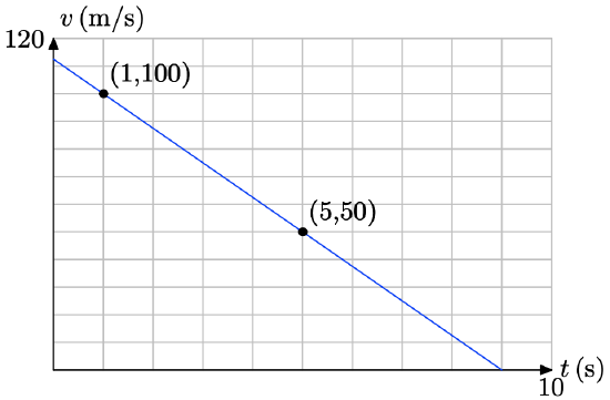
b) We’ll keep the units in our slope calculation to provide real-world meaning for the rate.
\[m = \dfrac{\delta v}{\delta t} = \dfrac{50 m/s − 100 m/s}{ 5 s − 1 s} = −12.5 (m/s)/s. \nonumber \]
That is, the slope is \(−12.5 m/s^2\). This is acceleration, the rate at which the speed is changing with respect to time. Every second, the speed decreases by 12.5 meters per second.
c) We use the point-slope form of the line, namely
\[y − y_{0} = m(x − x_{0}) \nonumber \]
However, v and t are taking the place of y and x, respectively, so the equation becomes \[v − v_{0} = m(t − t_{0}) \nonumber \], Now, substitute the slope m = −12.5 and the point \((t_{0}, v_{0}) = (1, 100)\) to obtain \[v − 100 = −12.5(t − 1) \nonumber \]. Solve this for v, obtaining \[v − 100 = −12.5t + 12.5 \\ v = −12.5t + 112.5 \nonumber \]. Equivalently, we could use function notation and write \[v(t) = −12.5t + 112.5 \nonumber \].
d) When the ball reaches its maximum height, its speed will equal zero. Consequently, to find the time of this event, we must solve v(t) = 0. Replace v(t) with −12.5t + 112.5 and solve for t. \[−12.5t + 112.5 = 0 \\ −12.5t = −112.5 \\ t = 9 \nonumber \]. Hence, it takes 9 seconds for the ball to reach its maximum height.
A ball is thrown vertically upward on a distant planet. After 2 seconds, its velocity is 320 feet per second. After 8 seconds, the velocity is 200 feet per second. Assume that the velocity v of the ball is a linear function of the time t.
a) On graph paper, sketch the graph of the velocity v versus the time t. Assume that the velocity is the dependent variable and place it on the vertical axis.
b) Determine the slope of the line, including its units, then give a real world explanation of the meaning of this slope.
c) Determine an equation that models the velocity v of the ball as a function of time t.
d) Determine the time it takes the ball to reach its maximum height.
An automobile is traveling down the autobahn and the driver applies its brakes. After 2 seconds, the car’s speed is 60 km/h. After 4 seconds, the car’s speed is 50 km/h.
a) On graph paper, sketch the graph of the velocity v versus the time t. Assume that the velocity is the dependent variable and place it on the vertical axis.
b) Determine the slope of the line, including its units, then give a real world explanation of the meaning of this slope.
c) Determine an equation that models the velocity v of the automobile as a function of time t. d) Determine the time it takes the automobile to stop.
- Answer
-
a) After 2 seconds, the speed of the car is 60 km/h. This is the point (2, 60). After 4 seconds, the car’s speed is 50 km/h. This is the point (4, 50). Plot these two points and draw a line through them, as shown in the plot below.
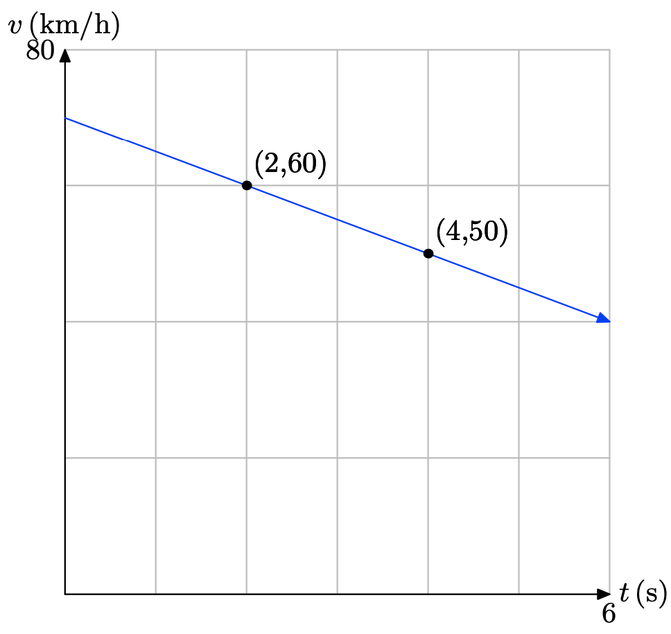
b) We’ll keep the units in our slope calculation to provide real-world meaning for the rate.
\[m = \dfrac{\delta v}{\delta t} = \dfrac{50 km/h − 60 km/h}{ 4 s − 2 s }= −5 (km/h)/s \nonumber \]
That is, the slope is −5 (km/h)/s. This is acceleration, the rate at which the speed is changing with respect to time. Every second, the speed decreases by 5 kilometers per hour.
c) We use the point-slope form of the line, namely \[y − y_{0} = m(x − x_{0}) \nonumber \], However, v and t are taking the place of y and x, respectively, so the equation becomes \[v − v_{0} = m(t − t_{0}) \nonumber \], Now, substitute the slope m = −5 and the point \((t_{0}, v_{0}) = (2, 60)\) to obtain \[v − 60 = −5(t − 2) \nonumber \]. Solve this for v, obtaining \[v − 60 = −5t + 10 \\ v = −5t + 70 \nonumber \]. Equivalently, we could use function notation and write \[v(t) = −5t + 70 \nonumber \].
d) To find the time it takes the car to stop, we must determine the time t so that \[v(t) = 0 \nonumber \]. Replace v(t) with −5t + 70 and solve for t.
\[−5t + 70 = 0\\ −5t = −70 \\ t = 14 \nonumber \]. Hence, it takes 14 seconds for the to brake to a stop.
An automobile is traveling down the autobahn and its driver steps on the accelerator. After 2 seconds, the car’s velocity is 30 km/h. After 4 seconds, the car’s velocity is 40 km/h.
a) On graph paper, sketch the graph of the velocity v versus the time t. Assume that the velocity is the dependent variable and place it on the vertical axis.
b) Determine the slope of the line, including its units, then give a real world explanation of the meaning of this slope.
c) Determine an equation that models the velocity v of the automobile as a function of time t.
d) Determine the speed of the vehicle after 8 seconds.
Suppose that the demand d for a particular brand of teakettle is a linear function of its unit price p. When the unit price is fixed at $30, the demand for teakettles is 100. This means the public buys 100 teakettles. If the unit price is fixed at $50, then the demand for teakettles is 60.
a) On graph paper, sketch the graph of the demand d versus the unit price p. Assume that the demand is the dependent variable and place it on the vertical axis.
b) Determine the slope of the line, including its units, then give a real world explanation of the meaning of this slope.
c) Determine an equation that models the demand d for teakettles as a function of unit price p.
d) Compute the demand if the unit price is set at $40.
- Answer
-
a) When the unit price is $30, the demand is 100 teakettles. This is the point (30, 100). When the unit price is $50, the demand is 60 teakettles. This is the point (50, 60). Plot the points (30, 100) and (50, 60) and draw a line through them, as shown in the plot below.
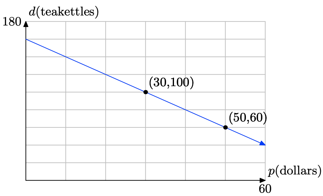
b) We’ll keep the units in our slope calculation to provide real-world meaning for the rate.
\[m = \dfrac{\delta d}{\delta p} = \dfrac{60 teakettles − 100 teakettles}{ 50 dollars − 30 dollars } = −2 teakettles/dollar \nonumber \]
That is, the slope is −2 teakettles/dollar. This is the rate at which the demand is changing with respect to the unit price. For every increase in the unit price of one dollar, the demand is lowered by 2 teakettles (2 fewer teakettles are bought).
c) We use the point-slope form of the line, namely\[ y − y_{0} = m(x − x_{0}) \nonumber \], However, d and p are taking the place of y and x, respectively, so the equation becomes
\[d − d_{0} = m(p − p_{0}) \nonumber \]
Now, substitute the slope m = −2 and the point \((p_{0}, d_{0}) = (30, 100)\) to obtain \[d − 100 = −2(p − 30) \nonumber \]. Solve this for d, obtaining
\[d − 100 = −2p + 60 \\ d = −2p + 160 \nonumber \]
Equivalently, we could use function notation and write d(p) = −2p + 160.
d) To determine the demand if the unit price is $40, compute \[ d(40) = −2(40) + 160 = 80 \nonumber \]
Hence, the demand is for 80 teakettles if the price per kettle is set at $40.
It’s perfect kite-flying weather on the coast of Oregon. Annie grabs her kite, climbs up on the roof of her two story home, and begins playing out kite string. In 10 seconds, Annie’s kite is 120 feet above the ground. After 20 seconds, it is 220 feet above the ground. Assume that the height h of the kite above the ground is a linear function of the amount of time t that has passed since Annie began playing out kite string.
a) On graph paper, sketch the graph of the height h of the kite above ground versus the time t . Assume that the height is the dependent variable and place it on the vertical axis.
b) Determine the slope of the line, including its units, then give a real world explanation of the meaning of this slope.
c) Determine an equation that models the height h of the kite as a function of time t.
d) Determine the height of the kite after 20 seconds.
e) Determine the height of Annie’s second story roof above ground.
3.5 Exercises
The following set of data about revolving consumer credit (debt) in the United States is from Google.com. This is primarily made up of credit card debt, but also includes other consumer non-mortgage credit, like those offered by commercial banks, credit unions, Sallie Mae, and the federal government.
| Year | yrs x after 2001 | all revolving credit C in billions of $ |
|---|---|---|
| 2001 | 0 | 721.0 |
| 2002 | 1 | 741.2 |
| 2003 | 2 | 759.3 |
| 2004 | 3 | 786.1 |
| 2005 | 4 | 805.4 |
a) Set up a coordinate system on graph paper, placing the credit C on the vertical axis, and the years x after 2001 on the horizontal axis. Label and scale each axis appropriately. Draw what you feel is the line of best fit. Remember to draw all lines with a ruler.
b) Select two points on your line of best fit that are not from the data table above. Use these two points to determine the slope of the line. Include units with your answer. Write a sentence or two explaining the real world significance of the slope of the line of best fit.
c) Use one of the two points on the line and the slope to determine the equation of the line of best fit in point-slope form. Use C and x for the dependent and independent variables, respectively. Solve the resulting equation for C and write your result using function notation.
d) Use the equation developed in part (c) to predict the revolving credit debt in the year 2008.
e) If the linear trend predicted by the line of best fit continues, in what year will the revolving credit debt reach 1.0 trillion dollars?
- Answer
-
a) Scale and label the axes, plot the points, then draw the line of best fit.

b) Select two points, P(1.4, 750) and Q(2.8, 780) that are points on the line but not points in the original data table.
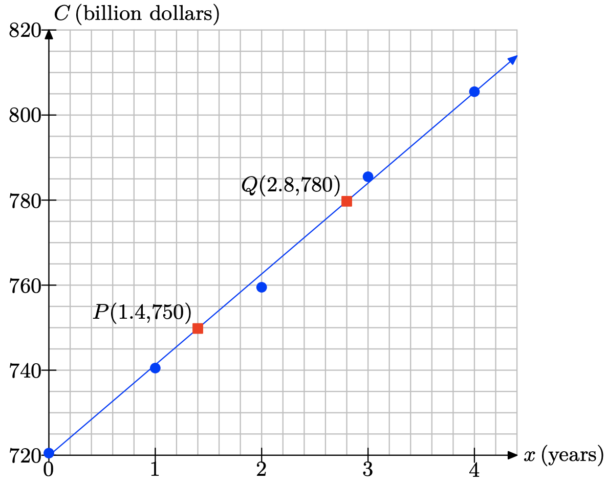
Use these two points to calculate the slope of the line of best fit.
\[m = \dfrac{\delta C}{\delta x} = \dfrac{780 − 750}{ 2.8 − 1.4} \nonumber \] billion dollars/year
Using a calculator, the slope is approximately 21.42 billion dollars per year. What this means is that the credit debt is increasing at a rate of 21.42 billion dollars per year. c) To find the equation of the line, use the point P(1.4, 750) and the slope m = 21.42 in the point-slope form of the line.
\[y − y_{0} = m(x − x_{0}) \\ y − 750 = 21.42(x − 1.4) \nonumber \]
Replace y and x with C and x, respectively, then solve for C in terms of x.
\[C − 750 = 21.42(x − 1.4) \\ C − 750 = 21.42x − 29.988 \\ C = 21.42x + 720.012 \nonumber \]
In function notation, C(x) = 21.42x + 720.012. Note: Answers will vary somewhat due to the subjective nature of drawing the line of best fit and picking points on the line.
d) The year 2008 gives x = 2008−2001 = 7 years since 2001. Hence, to find the credit debt in 2008, we use C(x) = 21.42x + 720.012 and evaluate
\[C(7) = 21.42(7) + 720.012 = 869.952 \nonumber \]
Hence, the credit debt in 2008 will be approximately 869 billion dollars.
e) A trillion dollars is 1000 billion dollars. Hence, to find when the credit debt is 1000 billion dollars, we must solve C(x) = 1000 for x.
\[C(x) = 1000 \\ 21.42x + 720.012 = 1000 \\ 21.42x = 279.988 \\ x \approx 13.07 \nonumber \] Hence, the credit debt will reach a trillion dollars approximately 13 years after the year 2001, or a little bit into the year 2014.
The following set of data about non-revolving credit (debt) in the United States is from Google.com. The largest component of non-revolving credit is automobile loans, but it is also includes student loans and other defined-term consumer loans.
| Year | yrs x after 2001 | Nonrevolving debt D in billions of $ |
|---|---|---|
| 2001 | 0 | 1121.3 |
| 2002 | 1 | 1184.1 |
| 2003 | 2 | 1247.3 |
| 2004 | 3 | 1305.0 |
| 2005 | 4 | 1342.3 |
a) Set up a coordinate system on graph paper, placing the non-revolving credit debt D on the vertical axis, and the years x after 2001 on the horizontal axis. Label and scale each axis appropriately. Draw what you feel is the line of best fit. Remember to draw all lines with a ruler.
b) Select two points on your line of best fit that are not from the data table above. Use these two points to determine the slope of the line. Include units with your answer. Write a sentence or two explaining the real world significance of the slope of the line of best fit.
c) Use one of the two points on the line and the slope to determine the equation of the line of best fit in pointslope form. Use D and x for the dependent and independent variables, respectively. Solve the resulting equation for D and write your result using function notation.
d) Use the equation developed in part (c) to predict the non-revolving credit debt in the year 2008. e) If the linear trend predicted by the line of best fit continues, in what year will the non-revolving credit debt reach 2.0 trillion dollars?
According to the U.S. Bureau of Transportation (www.bts.gov), retail sales of new cars declined every year from 2000- 2004, as shown in the following table.
| Year | yrs x after 2000 | Sales S in thousands |
|---|---|---|
| 2001 | 0 | 8847 |
| 2002 | 1 | 8423 |
| 2003 | 2 | 8103 |
| 2004 | 3 | 7610 |
| 2005 | 4 | 7506 |
a) Set up a coordinate system on graph paper, placing the sales S on the vertical axis, and the years x after 2000 on the horizontal axis. Label and scale each axis appropriately. Draw what you feel is the line of best fit. Remember to draw all lines with a ruler.
b) Select two points on your line of best fit that are not from the data table above. Use these two points to determine the slope of the line. Include units with your answer. Write a sentence or two explaining the real world significance of the slope of the line of best fit.
c) Use one of the two points on the line and the slope to determine the equation of the line of best fit in point-slope form. Use S and x for the dependent and independent variables, respectively. Solve the resulting equation for S and write your result using function notation.
d) Use the equation developed in part (c) to predict sales in the year 2006.
e) If the linear trend predicted by the line of best fit continues, when will sales drop to 7 million cars per year?
- Answer
-
a) Scale and label the axes, plot the points, then draw the line of best fit.
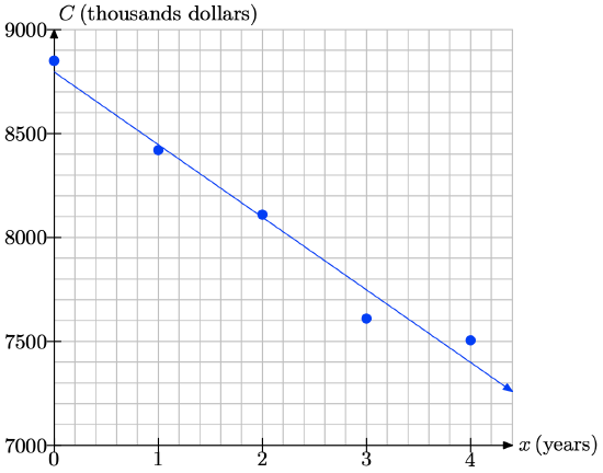
b) Select two points, P(1.4, 8300) and Q(4.0, 7400) that are points on the line but not points in the original data table.
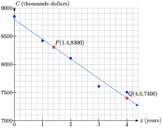
Use these two points to calculate the slope of the line of best fit.
\[m = \dfrac{\delta C }{\delta x} = \dfrac{8300 − 7400 }{4.0 − 1.4} \nonumber \] thousand cars/year Using a calculator, the slope is approximately −346.15 thousand cars per year. What this means is that sales of new cars is decreasing at an approximate rate of 346 thousand cars per year.
c) To find the equation of the line, use the point P(1.4, 8300) and the slope m = −346.15 in the point-slope form of the line.
\[y − y_{0} = m(x − x_{0}) \\ y − 8300 = −346.15(x − 1.4) \nonumber \]
Replace y and x with S and x, respectively, then solve for S in terms of x.
\[S − 8300 = −346.15(x − 1.4) \\ S − 8300 = −346.15x + 484.61 \\ S = −346.15x + 8784.61 \nonumber \]
In function notation, S(x) = −346.15x + 8784.61. Note: Answers will vary somewhat due to the subjective nature of drawing the line of best fit and picking points on the line.
d) To determine the sales in 2006, evaluate S(x) = −346.15x+8784.61 at x = 2006− 2000 = 6.
\[S(6) = −346.15(6) + 8784.61 = 6707.71 \nonumber \]
Thus, the sales will be approximately 6,707,710 new cars.
e) To determine when sales of new cars will drop to 7 million, we must solve
\[S(x) = 7000. −346.15x + 8784.61 = 7000 \\ −346.15x = −1784.61 \\ x \approx 5.16 \nonumber \]
Hence, sales will reach 7 million cars somewhere in the year 2005-2006.
The following table shows total midyear population of the world according to the U.S. Census Bureau, (www.census.gov) for recent years.
| Year | yrs x after 2000 | Population P in billions |
|---|---|---|
| 2000 | 0 | 6.08 |
| 2001 | 1 | 6.16 |
| 2002 | 2 | 6.23 |
| 2003 | 3 | 6.30 |
| 2004 | 4 | 6.38 |
| 2005 | 5 | 6.45 |
| 2006 | 6 | 6.53 |
a) Set up a coordinate system on graph paper, placing the population P on the vertical axis, and the years x after 2000 on the horizontal axis. Label and scale each axis appropriately. Draw what you feel is the line of best fit. Remember to draw all lines with a ruler.
b) Select two points on your line of best fit that are not from the data table above. Use these two points to determine the slope of the line. Include units with your answer. Write a sentence or two explaining the real world significance of the slope of the line of best fit.
c) Use one of the two points on the line and the slope to determine the equation of the line of best fit in point-slope form. Use P and x for the dependent and independent variables, respectively. Solve the resulting equation for P and write your result using function notation.
d) Use the equation developed in part (c) to predict the population in 2010.
e) If the linear trend predicted by the line of best fit continues, when will world population reach 7 billion?
The following table shows an excerpt from the U.S. Census Bureau’s 2005 data (www.census.gov) on annual sales of new homes in the United States.
| Price Range (thousands of $) | Number sold (thousands) |
|---|---|
| 150 − 199 | 246 |
| 200 − 249 | 200 |
| 250 − 299 | 152 |
We cannot use price ranges as coordinate values (we must have single values), so we replace each price range in the table with a single price in the middle of the range–the average value of a home in that range. This gives us the following modified table:
| Avg Price P (thousands of $) | Number sold N (thousands) |
|---|---|
| 175 | 246 |
| 225 | 200 |
| 275 | 152 |
We can now plot the data on a coordinate system.
a) Enter the data into your calculator and make a scatter plot. Copy it down onto your paper, labeling appropriately.
b) Use your calculator to determine a line of best fit. This is called a linear demand function, because it allows you to predict the demand for houses with a certain price. Write it using function notation and round to the nearest thousandth. Graph it on your calculator and copy it onto your coordinate system.
c) Use the linear demand function to predict annual sales of homes priced at $200, 000. Try to use the TABLE feature on your calculator to make this prediction.
- Answer
-
a) Select STAT, then 1:Edit and enter the data as shown in (a). Select 2nd STAT PLOT, then turn turn on Plot1 as shown in (b). Select scatterplot, choose the lists you used for the data, then a marker, as shown in (b). Finally, select 9:ZoomStat from the ZOOM menu to produce the plot in (c).
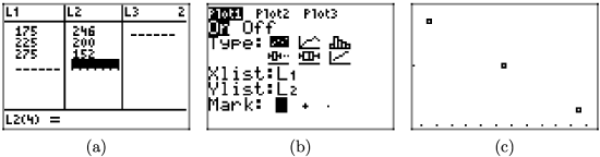
b) Push the STAT button, right-arrow to the CALC menu, then select 4:LinReg(ax+b), followed by L1, a comma, L2, a comma, and Y1 from the VARS menu (select Y-VARS then 1:Function submenus). The result is shown in (a). Press ENTER to produce the calculation shown in (b). This is the line of best fit. This procedure also stores the line of best fit in Y1, so pushing the GRAPH button produces the line of best fit shown in (c).
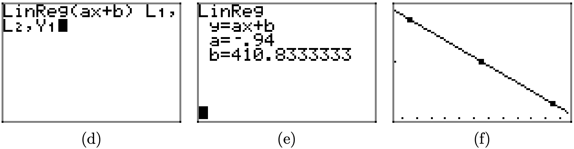
In (b) above, we see that the number sold N, as a function of average price P is given by the linear function N(P) = −0.94P + 410.833.
c) If all went well in part (b), then we can press 2nd TBL SET and set up the table parameters as shown in (g). Make sure the independent variable is set to ASK. Select 2nd TABLE, then enter 200 (which represents an average price p = $200, 000) as shown in (h).
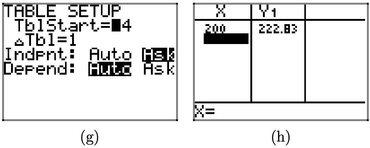
Thus, N(200) = 222.83, so approximately 222.83 thousand or 222, 830 homes are sold at the average price of $200,000.
The following table shows data from the National Association of Homebuilders (www.nahb.org), indicating the median price of new homes in the United States.
| Year | Median Price (thousands of $) |
|---|---|
| 2000 | 169 |
| 2001 | 175 |
| 2002 | 188 |
| 2003 | 195 |
| 2004 | 221 |
| 2005 | 238 |
a) Enter the data into your calculator and make a scatter plot. Copy it down onto your paper, labeling appropriately.
b) Use your calculator to determine a line of best fit that can be used to predict the median price of new homes in future years. Write it using function notation. Graph it on your calculator and copy it onto your coordinate system.
c) Use the linear demand function to predict the median price of a new home in 2010. Try to use the TABLE feature on your calculator to make this prediction.
d) Looking at the graph, do you think the linear demand function models the actual data points well? If not, why not? What does this mean about the prediction you made in part (c)?
Jim is hanging blocks of various mass on a spring in the physics lab. He notices that the spring will stretch further if he adds more mass to the end of the spring. He is soon convinced that the distance the spring will stretch depends on the amount of mass attached to it. He decides to take some measurements. He records the amount of mass attached to the end of the spring and then measures the distance that the spring stretched. Here is Jim’s data.
| Mass (grams) | Distance Stretched (cm) |
| 50 | 1.2 |
| 100 | 1.9 |
| 150 | 3.1 |
| 200 | 4.0 |
| 250 | 4.8 |
| 300 | 6.2 |
a) Enter the data into your calculator and make a scatter plot. Copy it down onto your paper, labeling appropriately.
b) Use your calculator to determine a line of best fit that can be used to predict the distance the spring stretches. Write it using function notation. Graph it on your calculator and copy it onto your coordinate system.
c) Use the function from part (c) to predict the distance the spring will stretch if 175 grams is attached to the spring. Try to use the TABLE feature on your calculator to make this prediction.
- Answer
-
a) Select STAT, then 1:Edit and enter the data as shown in (a). Select 2nd STAT PLOT, then turn turn on Plot1 as shown in (b). Select scatterplot, choose the lists you used for the data, then a marker, as shown in (b). Finally, select 9:ZoomStat from the ZOOM menu to produce the plot in (c).
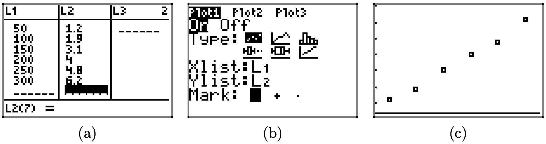
b) Push the STAT button, right-arrow to the CALC menu, then select 4:LinReg(ax+b), followed by L1, a comma, L2, a comma, and Y1 from the VARS menu (select Y-VARS then 1:Function submenus). The result is shown in (a). Press ENTER to produce the calculation shown in (b). This is the line of best fit. This procedure also stores the line of best fit in Y1, so pushing the GRAPH button produces the line of best fit shown in (c).
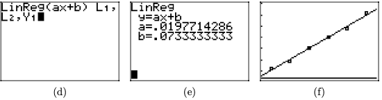
In (b) above, we see that the distance stretched d, as a function of mass m is given by the linear function d(m) = 0.01977m + 0.07333.
c) If all went well in part (b), then we can press 2nd TBL SET and set up the table parameters as shown in (g). Make sure the independent variable is set to ASK. Select 2nd TABLE, then enter 175 (which represents a mass of 175 grams) as shown in (h).
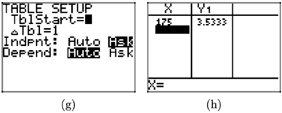
Thus, d(175) = 3.5333, so the spring stretches approximately 3.53 centimeters when a mass of 175 grams is attached.
Dave and Melody are lab partners in Tony Sartori’s afternoon chemistry lab. Professor Sartori has prepared an experiment to help them discover the relationship between the Celsius and Fahrenheit temperature scales. The experiment consists of a beaker full of ice and two thermometers, one calibrated in the Fahrenheit scale, the other in the Celsius scale. Dave and Melody use a Bunsen burner to heat the beaker, eventually bringing the water in the beaker to the boiling point. Every few minutees they make two temperature readings, one in Fahrenheit, one in Celsius. The data that they record during the laboratory session follows.
| Celsius | Fahrenheit |
|---|---|
| 4.0 | 39 |
| 18 | 65 |
| 30 | 85 |
| 51 | 122 |
| 70 | 159 |
| 85 | 186 |
| 100 | 210 |
a) Enter the data into your calculator and make a scatter plot. Copy it down onto your paper, labeling appropriately.
b) Use your calculator to determine a line of best fit that can be used to predict the Fahrenheit temperature as a function of the Celsius temperature. Write it using function notation. Graph it on your calculator and copy it onto your coordinate system.
c) Use the function from part (c) to predict the Fahrenheit temperature if the Celsius temperature is 40. Try to use the TABLE feature on your calculator to make this prediction.
d) Use the function from part (c) to predict the Celsius temperature if the Fahrenheit temperature is 100.
The following table shows data on home sales at the Mendocino Coast in 2005.
| Price Range (thousands of $) | Number sold (thousands) |
|---|---|
| 200 − 299 | 14 |
| 300 − 399 | 55 |
| 400 − 499 | 62 |
We cannot use price ranges as coordinate values (we must have single values), so we replace each price range in the table with a single price in the middle of the range–the average value of a home in that range. This gives us the following modified table:
| Avg Price P (thousands of $) | Number sold N (thousands) |
|---|---|
| 250 | 14 |
| 350 | 55 |
| 450 | 62 |
We can now plot the data on a coordinate system.
a) Enter the data into your calculator and make a scatter plot. Copy it down onto your paper, labeling appropriately.
b) Use your calculator to determine a line of best fit. Write it using function notation and round to the nearest thousandth. Graph it on your calculator and copy it onto your coordinate system.
c) Use the linear function to predict the sales for houses in the price range $500, 000− $599, 000. Use the average price of $550, 000 for this estimate.
d) The actual number of houses sold in the price range $500, 000 − $599, 000 was 41. Plot this as a point on your coordinate system and compare it to your linear function model’s prediction. Notice that this actual value is pretty different from the prediction.
e) What this means is that a linear model is not very good for the data for home sales! Draw a simple curve that goes through each of the data points. Notice that it does not very closely resemble the shape of a line! More sophisticated functions are required to model this example–such as quadratic functions, which we study in a later chapter. The moral of the story here is that not every data set can be modeled linearly!
- Answer
-
a) Select STAT, then 1:Edit and enter the data as shown in (a). Select 2nd STAT PLOT, then turn turn on Plot1 as shown in (b). Select scatterplot, choose the lists you used for the data, then a marker, as shown in (b). Finally, select 9:ZoomStat from the ZOOM menu to produce the plot in (c).
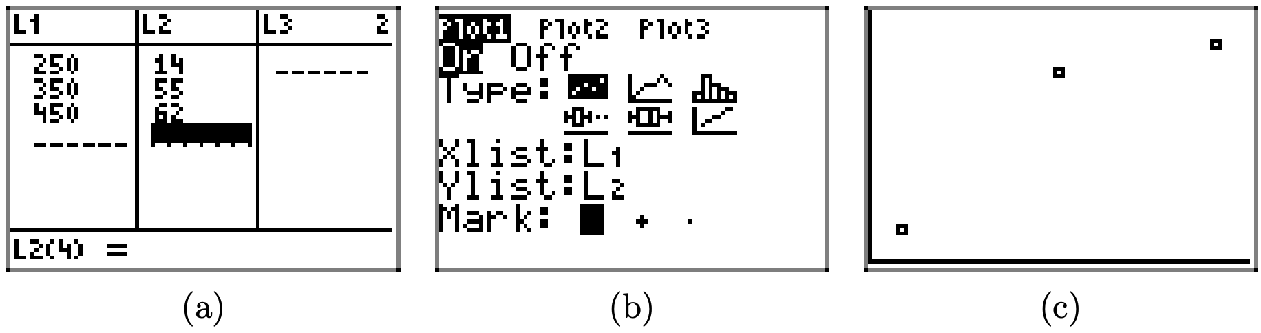
b) Push the STAT button, right-arrow to the CALC menu, then select 4:LinReg(ax+b), followed by L1, a comma, L2, a comma, and Y1 from the VARS menu (select Y-VARS then 1:Function submenus). The result is shown in (a). Press ENTER to produce the calculation shown in (b). This is the line of best fit. This procedure also stores the line of best fit in Y1, so pushing the GRAPH button produces the line of best fit shown in (c).
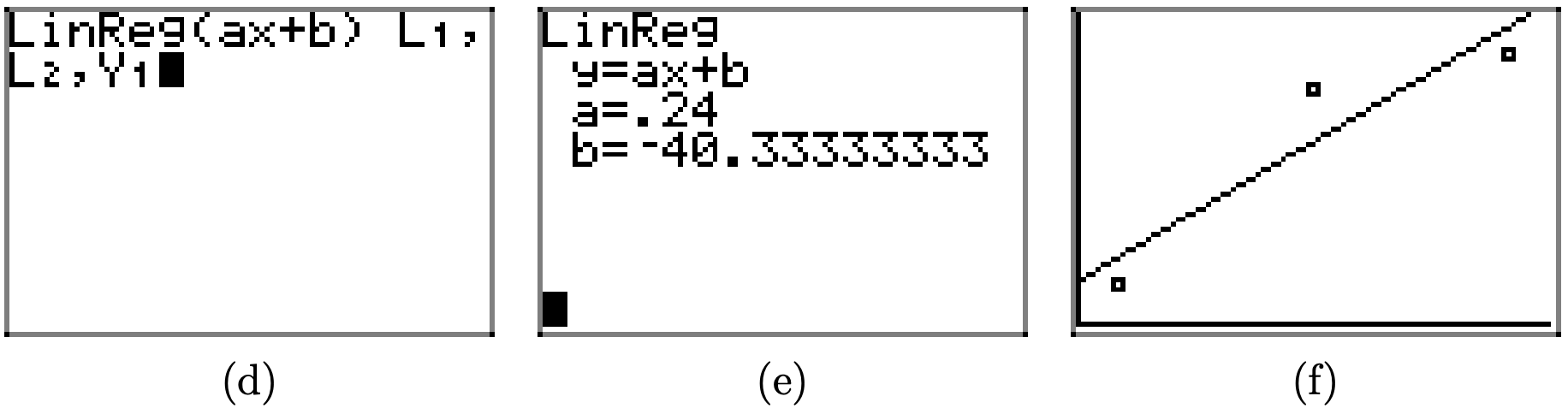
In (b) above, we see that the number sold N, as a function of average price P is given by the linear function N(P) = 0.24P − 40.33.
c) If all went well in part (b), then we can press 2nd TBL SET and set up the table parameters as shown in (g). Make sure the independent variable is set to ASK. Select 2nd TABLE, then enter 550 (which represents an average price P = $550, 000) as shown in (h).
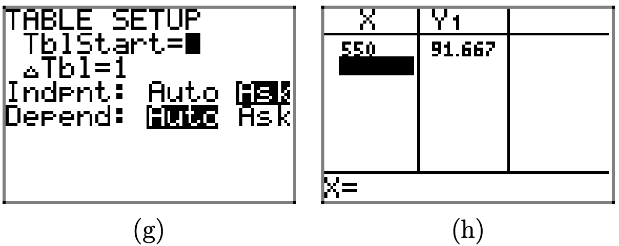
Thus, N(550) = 91.667, so approximately 91.667 thousand or 91, 667 homes are sold at the average price of $550,000. d) Press the STAT button, select 1:Edit and add the point (550, 41) to the table, as shown in (i). Select 9:ZoomStat from the ZOOM menu to produce the image in (j). Note that the data no longer depicts a linear trend, but something more of a nonlinear (curvy) nature
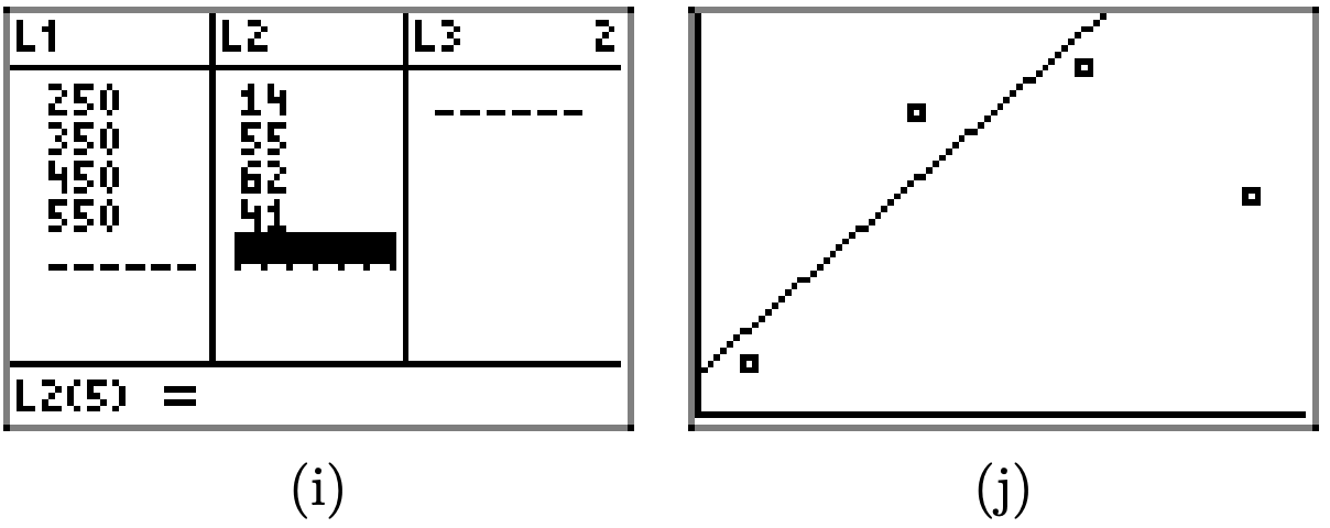
e) In (k) we’ve drawn a smooth curve of best fit.
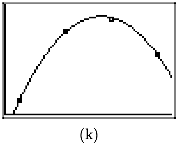
The following from the July 14, 2006 edition of the Beijing Today newspaper shows how high-heels affect the ball of the foot. The table shows the increase in percent of pressure on the ball of the foot for given heights of heels.
| Heel height h (inches) | %increase in pressure |
|---|---|
| 1 | 22 |
| 2 | 57 |
a) Enter the data into your calculator and make a scatter plot. Copy it down onto your paper, labeling appropriately.
b) Notice that, because we have exactly two data points, the line of best fit is the line that goes through both points. To begin finding the equation, use the slope formula to compute the slope.
c) Use the point-slope form to find an equation for the line. Write it in slope-intercept form.
d) Use the linear function to predict the percent of stress increase for a 3-inch heel.
e) The actual percent of pressure increase for a 3-inch heel is 76 %. Plot this as a point on your coordinate system and compare it to your linear function model’s prediction. Notice that this actual value is pretty different from the prediction.
f) What this means is that a linear model is not very good for the data! Draw a simple curve that goes through each of the data points. Notice that it does not very closely resemble the shape of a line! More sophisticated functions are required to model this example. Not every data set should be modeled linearly!