1.1: Introduction to Rⁿ

Calculus is the study of functional relationships and how related quantities change with each other. In your first exposure to calculus, the primary focus of your attention was on functions involving a single independent variable and a single dependent variable. For such a function \(f,\) a single real number input \(x\) determines a unique single output value \(f(x) .\) However, many of the functions of importance both within mathematics itself as well as in the application of mathematics to the rest of the world involve many variables simultaneously. For example, frequently in physics the function which describes the force acting on an object moving in space depends on three variables, the three coordinates which describe the location of the object. If the force function also varies with time, then the force depends on four variables. Moreover, the output of the force function will itself involve three variables, the three coordinate components of the force. Hence the force function is such that it takes three, or four, variables for input and outputs three variables. Far more complicated functions are easy to imagine: the gross national product of a country is a function of thousands of variables with a single variable as output, an airline schedule is a function with thousands of inputs (cities, planes, and people to be scheduled, as well as other variables like fuel costs and the schedules of competing airlines) and perhaps hundreds of outputs (the particular routes flown, along with their times). Although such functions may at first appear to be far more difficult to work with than the functions of single variable calculus, we shall see that we will often be able to reduce problems involving functions of several variables to related problems involving only single variable functions, problems which we may then handle using already familiar techniques.

By definition, a function takes a single input value and associates it with a single output value. Hence, even though in this book the inputs to our functions will often involve several variables, as will the outputs, we will nevertheless want to regard the input and output of a function as single points in some multidimensional space. This is natural in the case of, for example, the force function described above, where the input is a point in three dimensional space, four if we need to use time, but requires some mathematical abstraction if we want to consider the input to the gross national product function as a point in some space of many thousands of dimensions. Because even the geometry of two and three-dimensional space may be in some respects new to you, we will use this chapter to study the geometry of multidimensional space before proceeding to the study of calculus proper in Chapter 2.

Throughout the book we will let \(\mathbb{R}\) denote the set of real numbers.

Definition: Euclidean Space

By n-dimensional Euclidean space we mean the set

\[\mathbb{R}^{n}=\left\{\left(x_{1}, x_{2}, \ldots, x_{n}\right): x_{i} \in \mathbb{R}, i=1,2, \ldots, n\right\}.\]

That is, \(\mathbb{R}^{n}\) is the space of all ordered \(n\) -tuples of real numbers. We will denote a point in this space by

\[\mathbf{x}=\left(x_{1}, x_{2}, \ldots, x_{n}\right),\]

and, for \(i=1,2, \ldots, n,\) we call \(x_{i}\) the \(i\) th coordinate of \(\mathbf{x}\).

Example \(\PageIndex{1}\)

When \(n=2,\) we have

\[\mathbb{R}^{2}=\left\{\left(x_{1}, x_{2}\right): x_{1}, x_{2} \in \mathbb{R}\right\},\nonumber\]

which is our familiar representation for points in the Cartesian plane. As usual, we will in this case frequently label the coordinates as \(x\) and \(y,\) or something similar, instead of numbering them as \(x_{1}\) and \(x_{2}\).

Example \(\PageIndex{2}\)

When \(n=3,\) we have

\[\mathrm{R}^{3}=\left\{\left(x_{1}, x_{2}, x_{3}\right): x_{1}, x_{2}, x_{3} \in \mathrm{R}\right\}.\nonumber\]

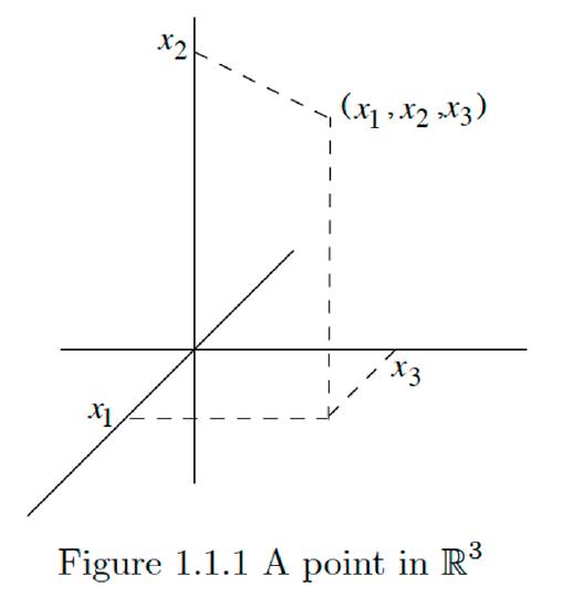
Just as we can think of \(\mathbb{R}^{2}\) as a way of assigning coordinates to points in the Euclidean plane, we can think of \(\mathbb{R}^{3}\) as assigning coordinates to three-dimensional Euclidean space. To picture this space, we must imagine three mutually perpendicular axes with the coordinates marked off along the axes as in Figure \(1.1 .1 .\) Again, we will frequently label the coordinates of a point in \(\mathbb{R}^{3}\) as, for example, \(x, y,\) and \(z,\) or \(u, v,\) and \(w,\) rather than using numbered coordinates.

Example \(\PageIndex{3}\)

If an object moves through space, its location may be specified with four coordinates, three spatial coordinate, say, \(x, y,\) and \(z,\) and one time coordinate, say \(t\) Thus its location is specified by a point \(\mathbf{p}=(x, y, z, t)\) in \(\mathbb{R}^{4} .\) Of course, we cannot draw a picture of such a point.

Before beginning our geometric study of \(\mathbb{R}^{n},\) we first need a few basic algebraic definitions.

Definition

Let \(\mathbf{x}=\left(x_{1}, x_{2}, \ldots, x_{n}\right)\) and \(\mathbf{y}=\left(y_{1}, y_{2}, \ldots, y_{n}\right)\) be points in \(\mathbf{R}^{n}\) and let \(a\) be a real number. Then we define

\[\mathbf{x}+\mathbf{y}=\left(x_{1}+y_{1}, x_{2}+y_{2}, \dots, x_{n}+y_{n}\right),\]

and

\[\mathbf{x}-\mathbf{y}=\left(x_{1}-y_{1}, x_{2}-y_{2}, \dots, x_{n}-y_{n}\right),\]

\[a \mathbf{x}=\left(a x_{1}, a x_{2}, \ldots, a x_{n}\right).\]

Example \(\PageIndex{4}\)

If \(x=(2,-3,1)\) and \(y=(-4,1,-2)\) are two points in \(R^{3},\) then

\[\begin{aligned} \mathbf{x}+\mathbf{y} &=(-2,-2,-1) \\ \mathbf{x}-\mathbf{y} &=(6,-4,3) \\ \mathbf{y}-\mathbf{x} &=(-6,4,-3) \\ 3 \mathbf{x} &=(6,-9,3), \end{aligned}\]

and

\[-2 y=(8,-2,4).\nonumber\]

Notice that we defined addition and subtraction for points in \(\mathbb{R}^{n},\) but we did not define multiplication. In general there is no form of multiplication for such points that is useful for our purpose. Of course, multiplication is defined in the special case \(n=1\) and for the special case \(n=2\) if we consider the points in \(\mathbb{R}^{2}\) as points in the complex plane. We shall see in Section 1.3 that there is also an interesting and useful type of multiplication in \(\mathbb{R}^{3} .\) Also note that \((1.1 .5)\) does provide a method for multiplying a point in \(\mathbb{R}^{n}\) by a real number, the result being another point in \(\mathrm{R}^{n}\). In such cases we often refer to the real number as a scalar and this multiplication as scalar multiplication. We shall provide a geometric interpretation of this form of multiplication shortly.

Geometry of \(\mathbb{R}^{n}\)

Recall that if \(\mathbf{x}=\left(x_{1}, x_{2}\right)\) and \(\mathbf{y}=\left(y_{1}, y_{2}\right)\) are two points in \(\mathbb{R}^{2},\) then, using the Pythagorean theorem, the distance from \(\mathbf{x}\) to \(\mathbf{y}\) is

\[\sqrt{\left(y_{1}-x_{1}\right)^{2}+\left(y_{2}-x_{2}\right)^{2}}.\nonumber\]

This formula is easily generalized to \(\mathbb{R}^{3}:\) Suppose \(\mathbf{x}=\left(x_{1}, x_{2}, x_{3}\right)\) and \(y=\left(y_{1}, y_{2}, y_{3}\right)\) are two points in \(\mathrm{R}^{3} .\) Let \(\mathbf{z}=\left(y_{1}, y_{2}, x_{3}\right) .\) Since the first two coordinates of \(\mathbf{y}\) and \(\mathbf{z}\) are the same, \(\mathbf{y}\) and \(\mathbf{z}\) lie on the same vertical line, and so the distance between them is simply

\[\left|y_{3}-x_{3}\right|.\]

Moreover, \(x\) and \(z\) have the same third coordinate, and so lie in the same horizontal plane. Hence the distance between \(\mathbf{x}\) and \(\mathbf{z}\) is the same as the distance between \(\left(x_{1}, x_{2}\right)\) and \(\left(y_{1}, y_{2}\right)\) in \(\mathbb{R}^{2},\) that is,

\[\sqrt{\left(y_{1}-x_{1}\right)^{2}+\left(y_{2}-x_{2}\right)^{2}}.\nonumber\]

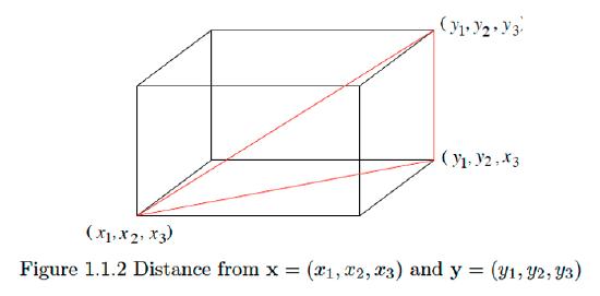
Finally, the points \(\mathbf{x}, \mathbf{y},\) and \(\mathbf{z}\) form a right triangle with right angle at \(\mathbf{z} .\) Hence, using the Pythagorean theorem again, the distance from \(x\) to \(y\) is

\[\sqrt{(\sqrt{\left(y_{1}-x_{1}\right)^{2}+\left(y_{2}-x_{2}\right)^{2}})^{2}+\left|y_{3}-x_{3}\right|^{2}}=\sqrt{\left(y_{1}-x_{1}\right)^{2}+\left(y_{2}-x_{2}\right)^{2}+\left(y_{3}-x_{3}\right)^{2}}.\nonumber\]

In particular, if we let \(\|x \|\) denote the distance from \(x=\left(x_{1}, x_{2}, x_{3}\right)\) to the origin \((0,0,0)\) in \(\mathbb{R}^{3},\) then

\[\|\mathbf{x}\|=\sqrt{x_{1}^{2}+x_{2}^{2}+x_{3}^{2}}.\nonumber\]

With this notation, the distance from \(\mathbf{x}\) to \(\mathbf{y}\) is

\[\begin{aligned}\|\mathbf{y}-\mathbf{x}\| &=\left\|\left(y_{1}-x_{1}, y_{2}-x_{2}, y_{3}-x_{3}\right)\right\| \\ &=\sqrt{\left(y_{1}-x_{1}\right)^{2}+\left(y_{2}-x_{2}\right)^{2}+\left(y_{3}-x_{3}\right)^{2}} \end{aligned} \]

Example \(\PageIndex{5}\)

If \(x=(1,2,-3)\) and \(y=(3,-2,1),\) then the distance from \(x\) to the origin is

\[\|\mathbf{x}\|=\sqrt{1^{2}+2^{2}+(-3)^{2}}=\sqrt{14}\nonumber\]

and the distance from \(x\) to \(y\) is given by

\[\|\mathbf{y}-\mathbf{x}\|=\|(2,-4,4)\|=\sqrt{4+16+16}=6.\nonumber\]

Although we do not have any physical analogies to work with when \(n>3,\) nevertheless we may generalize \((1.1 .9)\) in order to define distance in \(\mathbb{R}^{n}\).

Definition

If \(x=\left(x_{1}, x_{2}, \ldots, x_{n}\right)\) is a point in \(\mathbb{R}^{n},\) we define the norm of \(x,\) denoted \(\|\mathbf{x}\|,\) by

\[\|\mathbf{x}\|=\sqrt{x_{1}^{2}+x_{2}^{2}+\cdots+x_{n}^{2}}.\nonumber\]

For two points \(\mathbf{x}\) and \(\mathbf{y}\) in \(\mathbb{R}^{n},\) we define the distance between \(\mathbf{x}\) and \(\mathbf{y},\) denoted \(d(\mathbf{x}, \mathbf{y})\)

by

\[d(\mathbf{x}, \mathbf{y})=\|\mathbf{y}-\mathbf{x}\|.\nonumber\]

We will let \(\mathbf{0}=(0,0, \ldots, 0)\) denote the origin in \(\mathbb{R}^{n} .\) Then we have

\[\|\mathbf{x}\|=d(\mathbf{x}, \mathbf{0});\nonumber\]

that is, the norm of \(x\) is the distance from \(x\) to the origin.

Example \(\PageIndex{6}\)

If \(x=(2,3,-1,5),\) a point in \(\mathbb{R}^{4},\) then the distance from \(x\) to the origin is

\[\|\mathbf{x}\|=\sqrt{4+9+1+25}=\sqrt{39}.\nonumber\]

If \(\mathbf{y}=(3,2,1,4),\) then the distance from \(\mathbf{x}\) to \(\mathbf{y}\) is

\[d(\mathbf{x}, \mathbf{y})=\|\mathbf{y}-\mathbf{x}\|=\|(1,-1,2,-1)\|=\sqrt{7}.\nonumber\]

Note that if \(\mathbf{x}=\left(x_{1}, x_{2}, \ldots, x_{n}\right)\) is a point in \(\mathbb{R}^{n}\) and \(a\) is a scalar, then

\[\begin{aligned} \|a \mathbf{x}\| &=\left\|\left(a x_{1}, a x_{2}, \ldots, a x_{n}\right)\right\| \\ &=\sqrt{a^{2} x_{1}^{2}+a^{2} x_{2}^{2}+\cdots+a^{2}x_{n}^{2}} \\ &=|a| \sqrt{x_{1}^{2}+x_{2}^{2}+\cdots+x_{n}^{2}} \\ &=|a|\|\mathbf{x}\|.\end{aligned}\]

That is, the norm of a scalar multiple of \(x\) is just the absolute value of the scalar times the norm of \(\mathbf{x}\). In particular, if \(\mathbf{x} \neq \mathbf{0},\) then

\[\left\|\frac{1}{\|\mathbf{x}\|} \mathbf{x}\right\|=\frac{1}{\|\mathbf{x}\|}\|\mathbf{x}\|=1.\nonumber\]

That is,

\[\frac{1}{\|\mathbf{x}\|} \mathbf{x}\nonumber\]

is a unit distance from the origin.

Definition

Let \(\mathbf{p}=\left(p_{1}, p_{2}, \ldots, p_{n}\right)\) be a point in \(\mathbb{R}^{n}\) and let \(r>0\) be a real number. The set of all points \(\left(x_{1}, x_{2}, \ldots, x_{n}\right)\) in \(\mathbb{R}^{n}\) which satisfy the equation

\[\left(x_{1}-p_{1}\right)^{2}+\left(x_{2}-p_{2}\right)^{2}+\cdots+\left(x_{n}-p_{n}\right)^{2}=r^{2}\]

is called an \((n-1)-\) dimensional sphere with radius \(r\) and center \(\mathbf{p},\) which we denote \(S^{n-1}(\mathbf{p}, r) .\) The set of all points \(\left(x_{1}, x_{2}, \ldots, x_{n}\right)\) in \(\mathbb{R}^{n}\) which satisfy the inequality

\[\left(x_{1}-p_{1}\right)^{2}+\left(x_{2}-p_{2}\right)^{2}+\cdots+\left(x_{n}-p_{n}\right)^{2}<r^{2}\]

is called an open \(n\) -dimensional ball with radius \(r\) and center \(\mathbf{p},\) which we denote \(B^{n}(\mathbf{p}, r)\) The set of all points \(\left(x_{1}, x_{2}, \ldots, x_{n}\right)\) in \(\mathbb{R}^{n}\) which satisfy the inequality

\[\left(x_{1}-p_{1}\right)^{2}+\left(x_{2}-p_{2}\right)^{2}+\cdots+\left(x_{n}-p_{n}\right)^{2} \leq r^{2}\]

is called a closed n-dimensional ball with radius \(r\) and center \(\mathbf{P},\) which we denote \(\bar{B}^{n}(\mathbf{p}, r)\)

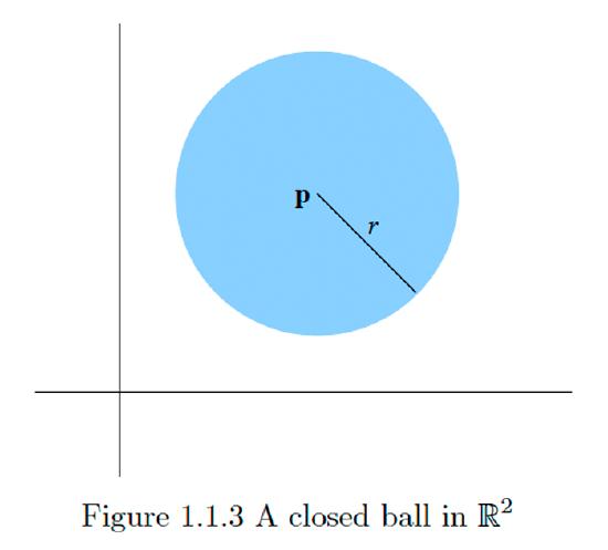
A sphere \(S^{n-1}(\mathbf{p}, r)\) is the set of all points which lie a fixed distance \(r\) from a fixed point \(\mathbf{p}\) in \(\mathbb{R}^{n}\). Note that for \(n=1, S^{0}(\mathbf{p}, r)\) consists of only two points, namely, the point \(\mathbf{p}-r\) that lies a distance \(r\) to the left of \(\mathbf{p}\) and the point \(\mathbf{p}+r\) that lies a distance \(r\) to the right of \(\mathbf{p} ; B^{1}(\mathbf{p}, r)\) is the open interval \((\mathbf{p}-r, \mathbf{p}+r) ;\) and \(\bar{B}^{1}(\mathbf{p}, r)\) is the closed interval \([\mathbf{p}-r, \mathbf{p}+r] .\) In this sense open and closed balls are natural analogs of open and closed intervals on the real line. For \(n=2,\) a sphere is a circle, an open ball is a disk without its enclosing circle, and a closed ball is a disk along with its enclosing circle.

Vectors

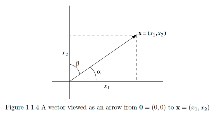
Many of the quantities of interest in physics, such as velocities, accelerations, and forces, involve both a magnitude and a direction. For example, we might speak of a force of magnitude 10 newtons acting on an object at the origin in a plane at an angle of \(\frac{\pi}{4}\) with the horizontal. It is common to picture such a quantity as an arrow, with length given by the magnitude and with the tip pointing in the specified direction, and to refer to it as 8 vector. Now any point \(\mathbf{x}=\left(x_{1}, x_{2}\right), \mathbf{x} \neq \mathbf{0},\) in \(\mathbb{R}^{2}\) specifies a vector in the plane, namely the vector starting at the origin and ending at \(\mathbf{x}\). The magnitude, or length, of such vector is \(\|\mathbf{x}\|\) and its direction is specified by the angle \(\alpha\) that it makes with the horizontal axis or by the angle \(\beta\) that it makes with the vertical axis. Note that

\[\cos (\alpha)=\frac{x_{1}}{\|x\|}\nonumber\]

and

\[\cos (\beta)=\frac{x_{2}}{\|x\|}\nonumber\]

and that, although neither \(\cos (\alpha)\) nor \(\cos (\beta)\) uniquely determines the direction of the vector by itself, together they completely determine the direction. See Figure 1.1.4.

In general, we may think of \(\mathbf{x}=\left(x_{1}, x_{2}, \ldots, x_{n}\right)\) either as a point in \(\mathbb{R}^{n}\) or as a vector in \(\mathbb{R}^{n},\) starting at the origin with length \(\|\mathbf{x}\| .\) If \(\mathbf{x} \neq \mathbf{0},\) we say, in analogy with the case in

\(\mathrm{R}^{2},\) that the direction of \(\mathrm{x}\) is the vector

\[\mathbf{u}=\left(\frac{x_{1}}{\|\mathbf{x}\|}, \frac{x_{2}}{\|\mathbf{x}\|}, \ldots, \frac{x_{n}}{\|\mathbf{x}\|}\right)\nonumber\]

The coordinates of this vector \(\mathbf{u}\) are called the direction cosines of \(\mathbf{x}\) because we may think of

\[u_{k}=\frac{x_{k}}{\|x\|} \nonumber\]

as the cosine of the angle between the vector \(x\) and the \(k\) th axis for \(k=1,2, \ldots, n,\) an interpretation that will become clearer after our discussion of angles in \(\mathbb{R}^{n}\) in the next section. Alternatively, we may think of \(\mathbf{u}\) as a vector of unit length that points in the same direction as \(\mathbf{x}\). Any vector of length \(1,\) such as \(\mathbf{u},\) is called a unit vector. We call \(\mathbf{0}\) the zero-vector since it has length 0. Note that 0 does not have a direction.

Example \(\PageIndex{7}\)

The vector \(\mathbf{x}=(1,2,-2,3)\) in \(\mathbf{R}^{4}\) has length \(\|\mathbf{x}\|=\sqrt{18}\) and direction

\[\mathbf{u}=\left(\frac{1}{\sqrt{18}}, \frac{2}{\sqrt{18}},-\frac{2}{\sqrt{18}}, \frac{3}{\sqrt{18}}\right)=\frac{1}{\sqrt{18}}(1,2,-2,3)\nonumber\]

It is now possible to give geometric meanings to our definitions of scalar multiplication, vector addition, and vector subtraction. First note that if \(\mathbf{x} \neq \mathbf{0}\) and \(a>0,\) then

\[\|a \mathbf{x}\|=a\|\mathbf{x}\|,\nonumber\]

so a \(\mathbf{x}\) has direction

\[\frac{1}{\|a \mathbf{x}\|} a \mathbf{x}=\frac{1}{\|\mathbf{x}\|} \mathbf{x}\nonumber\]

the same as \(\mathbf{x}\). Hence \(a \mathbf{x}\) points in the same direction as \(\mathbf{x},\) but with length \(a\) times the length of \(\mathbf{x} .\) If \(a<0,\) then

\[\|a \mathbf{x}\|=|a|\|\mathbf{x}\|=-a\|\mathbf{x}\|,\nonumber\]

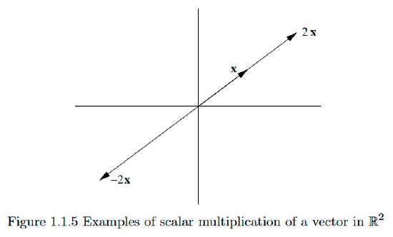
so \(a x\) has direction

\[\frac{1}{\|a \mathbf{x}\|} a \mathbf{x}=-\frac{1}{\|\mathbf{x}\|} \mathbf{x}.\nonumber\]

Hence, in this case, \(a x\) has the opposite direction of \(x\) with \(|a|\) times the length of x. See Figure 1.1.5 for examples in \(\mathbb{R}^{2}\).
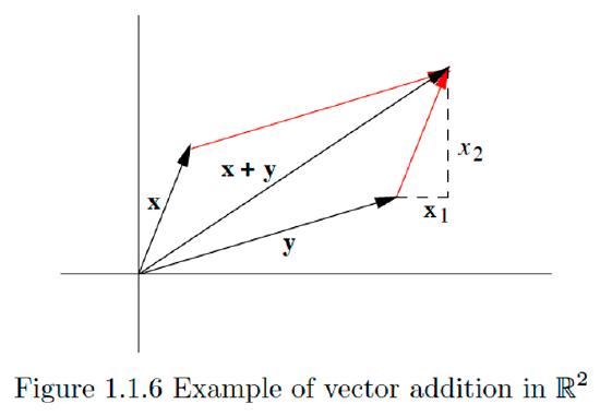
Next consider two vectors \(\mathbf{x}=\left(x_{1}, x_{2}\right)\) and \(\mathbf{y}=\left(y_{1}, y_{2}\right)\) in \(\mathbb{R}^{2}\) and their sum
\[\mathbf{z}=\mathbf{x}+\mathbf{y}=\left(x_{1}+y_{1}, x_{2}+y_{2}\right).\nonumber\]

Note that the tip of \(\mathbf{z}\) is located \(x_{1}\) units horizontally and \(x_{2}\) units vertically from the tip of \(\mathbf{y} .\) Geometrically, the tip of \(\mathbf{z}\) is located at the tip of \(\mathbf{x}\) if \(\mathbf{x}\) were first translated parallel to itself so that its tail now coincided with the tip of \(\mathbf{y} .\) Equivalently, we can view \(\mathbf{z}\) as the diagonal of the parallelogram which has \(\mathbf{x}\) and \(\mathbf{y}\) for its sides. See Figure 1.1.6 for an example.

Finally, consider two vectors \(\mathbf{x}=\left(x_{1}, x_{2}\right)\) and \(\mathbf{y}=\left(y_{1}, y_{2}\right)\) in \(\mathbb{R}^{2}\) and their difference

\[\mathbf{z}=\mathbf{x}-\mathbf{y}=\left(x_{1}-y_{1}, x_{2}-y_{2}\right).\]

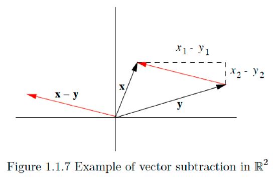
Note that since the coordinates of \(\mathbf{z}\) are just the differences in the coordinates of \(\mathbf{x}\) and \(\mathbf{y}\), \(\mathbf{z}\) has the magnitude and direction of an arrow pointing from the tip of \(\mathbf{y}\) to the tip of \(\mathbf{x}\), as illustrated in Figure \(1.1 .7 .\) In other words, we may picture \(\mathbf{z}\) geometrically by translating an arrow drawn from the tip of \(\mathbf{y}\) to the tip of \(\mathbf{z}\) parallel to itself until its tail is at the origin.

In the previous discussion it is tempting to think of the arrow from the tip of \(\mathbf{y}\) to the tip of \(\mathbf{x}\) as really being \(\mathbf{x}-\mathbf{y},\) not just a parallel translate of \(\mathbf{x}-\mathbf{y} .\) In fact, it is convenient and useful to think of parallel translates of a given vector, that is, vectors which have the same direction and magnitude, but with their tails not at the origin, as all being the same vector, just drawn in different places in space. We shall see many instances where viewing vectors in this way significantly helps our understanding.

Before closing this section, we need to call attention to some special vectors.

Definition: Standard Basis Vectors

The vectors

\[\begin{array}{l}{\mathbf{e}_{1}=(1,0,0, \ldots, 0)} \\ {\mathbf{e}_{2}=(0,1,0, \ldots, 0)} \\ {\vdots} \\ {\mathbf{e}_{n}=(0,0,0, \ldots, 1)}\end{array}\]

in \(\mathbb{R}^{n}\) are called the standard basis vectors.

Example \(\PageIndex{8}\)

In \(\mathbb{R}^{2}\) the standard basis vectors are \(\mathbf{e}_{1}=(1,0)\) and \(\mathbf{e}_{2}=(0,1) .\) Note that if \(\mathbf{x}=(x, y)\) is any vector in \(\mathbb{R}^{2},\) then

\[\mathbf{x}=(x, 0)+(0, y)=x(1,0)+y(0,1)=x \mathbf{e}_{1}+y e_{2}. \nonumber\]

For example, \((2,5)=2 \mathrm{e}_{1}+5 \mathrm{e}_{2}\).

Example \(\PageIndex{9}\)

In \(\mathbb{R}^{3}\) the standard basis vectors are \(\mathrm{e}_{1}=(1,0,0), \mathrm{e}_{2}=(0,1,0),\) and \(\mathrm{e}_{3}=\) \((0,0,1) .\) Note that if \(\mathbf{x}=(x, y, z)\) is any vector in \(\mathbb{R}^{3},\) then

\[\mathbf{x}=(x, 0,0)+(0, y, 0)+(0,0, z)=x(1,0,0)+y(0,1,0)+z(0,0,1)=x e_{1}+y e_{2}+z e_{3}\nonumber\]

For example, \((1,2,-4)=\mathbf{e}_{1}+2 \mathbf{e}_{2}-4 \mathbf{e}_{3}\).

The previous two examples are easily generalized to show that any vector in \(\mathrm{R}^{n}\) may be written as a sum of scalar multiples of the standard basis vectors. Specifically, if \(\mathbf{x}=\left(x_{1}, x_{2}, \ldots, x_{n}\right),\) then we may write \(\mathbf{x}\) as

\[\mathbf{x}=x_{1} \mathbf{e}_{1}+x_{2} \mathbf{e}_{2}+\cdots+x_{n} \mathbf{e}_{n}.\]

We say that \(x\) is a linear combination of the standard basis vectors \(e_{1}, e_{2}, \ldots, e_{n} .\) It is also important to note that there is only one choice for the scalars in this linear combination. That is, for any vector \(\mathbf{x}\) in \(\mathbb{R}^{n}\) there is one and only one way to write \(\mathbf{x}\) as a linear combination of the standard basis vectors.

Notes on notation

In this text, we will denote vectors using a plain bold font. This is a common convention, but not the only one used for denoting vectors. Another frequently used convention is to place arrows above a variable which denotes a vector. For example, one might write \(\vec{x}\) for what we have been denoting \(\mathbf{x}\).

It is also worth noting that in many books the standard basis vectors in \(\mathbb{R}^{2}\) are denoted by i and \(\mathbf{j}(\text { or } \vec{i} \text { and } \vec{j}),\) and the standard basis vectors in \(\mathbb{R}^{3}\) by \(\mathbf{i}, \mathbf{j},\) and \(\mathbf{k}\) (or \(\vec{i}, \vec{j},\) and \(\vec{k}\) ). Since this notation is not easy to extend to higher dimensions, we will not make much use of it.