7.02: Trapezoidal Rule of Integration
- Page ID
- 126423
\( \newcommand{\vecs}[1]{\overset { \scriptstyle \rightharpoonup} {\mathbf{#1}} } \)
\( \newcommand{\vecd}[1]{\overset{-\!-\!\rightharpoonup}{\vphantom{a}\smash {#1}}} \)
\( \newcommand{\dsum}{\displaystyle\sum\limits} \)
\( \newcommand{\dint}{\displaystyle\int\limits} \)
\( \newcommand{\dlim}{\displaystyle\lim\limits} \)
\( \newcommand{\id}{\mathrm{id}}\) \( \newcommand{\Span}{\mathrm{span}}\)
( \newcommand{\kernel}{\mathrm{null}\,}\) \( \newcommand{\range}{\mathrm{range}\,}\)
\( \newcommand{\RealPart}{\mathrm{Re}}\) \( \newcommand{\ImaginaryPart}{\mathrm{Im}}\)
\( \newcommand{\Argument}{\mathrm{Arg}}\) \( \newcommand{\norm}[1]{\| #1 \|}\)
\( \newcommand{\inner}[2]{\langle #1, #2 \rangle}\)
\( \newcommand{\Span}{\mathrm{span}}\)
\( \newcommand{\id}{\mathrm{id}}\)
\( \newcommand{\Span}{\mathrm{span}}\)
\( \newcommand{\kernel}{\mathrm{null}\,}\)
\( \newcommand{\range}{\mathrm{range}\,}\)
\( \newcommand{\RealPart}{\mathrm{Re}}\)
\( \newcommand{\ImaginaryPart}{\mathrm{Im}}\)
\( \newcommand{\Argument}{\mathrm{Arg}}\)
\( \newcommand{\norm}[1]{\| #1 \|}\)
\( \newcommand{\inner}[2]{\langle #1, #2 \rangle}\)
\( \newcommand{\Span}{\mathrm{span}}\) \( \newcommand{\AA}{\unicode[.8,0]{x212B}}\)
\( \newcommand{\vectorA}[1]{\vec{#1}} % arrow\)
\( \newcommand{\vectorAt}[1]{\vec{\text{#1}}} % arrow\)
\( \newcommand{\vectorB}[1]{\overset { \scriptstyle \rightharpoonup} {\mathbf{#1}} } \)
\( \newcommand{\vectorC}[1]{\textbf{#1}} \)
\( \newcommand{\vectorD}[1]{\overrightarrow{#1}} \)
\( \newcommand{\vectorDt}[1]{\overrightarrow{\text{#1}}} \)
\( \newcommand{\vectE}[1]{\overset{-\!-\!\rightharpoonup}{\vphantom{a}\smash{\mathbf {#1}}}} \)
\( \newcommand{\vecs}[1]{\overset { \scriptstyle \rightharpoonup} {\mathbf{#1}} } \)
\(\newcommand{\longvect}{\overrightarrow}\)
\( \newcommand{\vecd}[1]{\overset{-\!-\!\rightharpoonup}{\vphantom{a}\smash {#1}}} \)
\(\newcommand{\avec}{\mathbf a}\) \(\newcommand{\bvec}{\mathbf b}\) \(\newcommand{\cvec}{\mathbf c}\) \(\newcommand{\dvec}{\mathbf d}\) \(\newcommand{\dtil}{\widetilde{\mathbf d}}\) \(\newcommand{\evec}{\mathbf e}\) \(\newcommand{\fvec}{\mathbf f}\) \(\newcommand{\nvec}{\mathbf n}\) \(\newcommand{\pvec}{\mathbf p}\) \(\newcommand{\qvec}{\mathbf q}\) \(\newcommand{\svec}{\mathbf s}\) \(\newcommand{\tvec}{\mathbf t}\) \(\newcommand{\uvec}{\mathbf u}\) \(\newcommand{\vvec}{\mathbf v}\) \(\newcommand{\wvec}{\mathbf w}\) \(\newcommand{\xvec}{\mathbf x}\) \(\newcommand{\yvec}{\mathbf y}\) \(\newcommand{\zvec}{\mathbf z}\) \(\newcommand{\rvec}{\mathbf r}\) \(\newcommand{\mvec}{\mathbf m}\) \(\newcommand{\zerovec}{\mathbf 0}\) \(\newcommand{\onevec}{\mathbf 1}\) \(\newcommand{\real}{\mathbb R}\) \(\newcommand{\twovec}[2]{\left[\begin{array}{r}#1 \\ #2 \end{array}\right]}\) \(\newcommand{\ctwovec}[2]{\left[\begin{array}{c}#1 \\ #2 \end{array}\right]}\) \(\newcommand{\threevec}[3]{\left[\begin{array}{r}#1 \\ #2 \\ #3 \end{array}\right]}\) \(\newcommand{\cthreevec}[3]{\left[\begin{array}{c}#1 \\ #2 \\ #3 \end{array}\right]}\) \(\newcommand{\fourvec}[4]{\left[\begin{array}{r}#1 \\ #2 \\ #3 \\ #4 \end{array}\right]}\) \(\newcommand{\cfourvec}[4]{\left[\begin{array}{c}#1 \\ #2 \\ #3 \\ #4 \end{array}\right]}\) \(\newcommand{\fivevec}[5]{\left[\begin{array}{r}#1 \\ #2 \\ #3 \\ #4 \\ #5 \\ \end{array}\right]}\) \(\newcommand{\cfivevec}[5]{\left[\begin{array}{c}#1 \\ #2 \\ #3 \\ #4 \\ #5 \\ \end{array}\right]}\) \(\newcommand{\mattwo}[4]{\left[\begin{array}{rr}#1 \amp #2 \\ #3 \amp #4 \\ \end{array}\right]}\) \(\newcommand{\laspan}[1]{\text{Span}\{#1\}}\) \(\newcommand{\bcal}{\cal B}\) \(\newcommand{\ccal}{\cal C}\) \(\newcommand{\scal}{\cal S}\) \(\newcommand{\wcal}{\cal W}\) \(\newcommand{\ecal}{\cal E}\) \(\newcommand{\coords}[2]{\left\{#1\right\}_{#2}}\) \(\newcommand{\gray}[1]{\color{gray}{#1}}\) \(\newcommand{\lgray}[1]{\color{lightgray}{#1}}\) \(\newcommand{\rank}{\operatorname{rank}}\) \(\newcommand{\row}{\text{Row}}\) \(\newcommand{\col}{\text{Col}}\) \(\renewcommand{\row}{\text{Row}}\) \(\newcommand{\nul}{\text{Nul}}\) \(\newcommand{\var}{\text{Var}}\) \(\newcommand{\corr}{\text{corr}}\) \(\newcommand{\len}[1]{\left|#1\right|}\) \(\newcommand{\bbar}{\overline{\bvec}}\) \(\newcommand{\bhat}{\widehat{\bvec}}\) \(\newcommand{\bperp}{\bvec^\perp}\) \(\newcommand{\xhat}{\widehat{\xvec}}\) \(\newcommand{\vhat}{\widehat{\vvec}}\) \(\newcommand{\uhat}{\widehat{\uvec}}\) \(\newcommand{\what}{\widehat{\wvec}}\) \(\newcommand{\Sighat}{\widehat{\Sigma}}\) \(\newcommand{\lt}{<}\) \(\newcommand{\gt}{>}\) \(\newcommand{\amp}{&}\) \(\definecolor{fillinmathshade}{gray}{0.9}\)Lesson 1: Single-Application Trapezoidal Rule
Learning Objectives
After successful completion of this lesson, you should be able to:
1) derive the trapezoidal rule of integration,
2) use the trapezoidal rule of integration to solve problems,
Introduction
The trapezoidal rule is based on the Newton-Cotes formula that if one approximates the integrand by an \(n^{th}\) order polynomial, then the integral of the function is approximated by the integral of that \(n^{th}\) order polynomial. Integrating polynomials is simple and is based on the calculus formula.
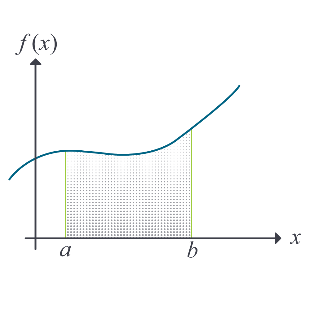
\[\int_{a}^{b} x^{n} \ dx = \left( \frac{b^{n + 1} - a^{n + 1}}{n + 1} \right),n \neq - 1\;\;\;\;\;\;\;\;\;\;\;\; (\PageIndex{1.1}) \nonumber\]
So if we want to approximate the integral
\[I = \int_{a}^{b} f(x) \ dx\;\;\;\;\;\;\;\;\;\;\;\; (\PageIndex{1.2}) \nonumber\]
to find the value of the above integral, one assumes
\[f(x) \approx f_{n}(x) \nonumber\]
where
\[f_{n}(x) = a_{0} + a_{1}x +\ldots + a_{n - 1}x^{n - 1} + a_{n}x^{n}.\;\;\;\;\;\;\;\;\;\;\;\; (\PageIndex{1.3}) \nonumber\]
where \(f_{n}(x)\) is a \(n^{th}\) order polynomial. The trapezoidal rule assumes \(n = 1\), that is, approximating the integral by a linear polynomial (straight line),
\[\int_{a}^{b} f(x) \ dx \approx \int_{a}^{b} f_{1}(x) \ dx\;\;\;\;\;\;\;\;\;\;\;\; (\PageIndex{1.4}) \nonumber\]
Method 1: Derived from Calculus
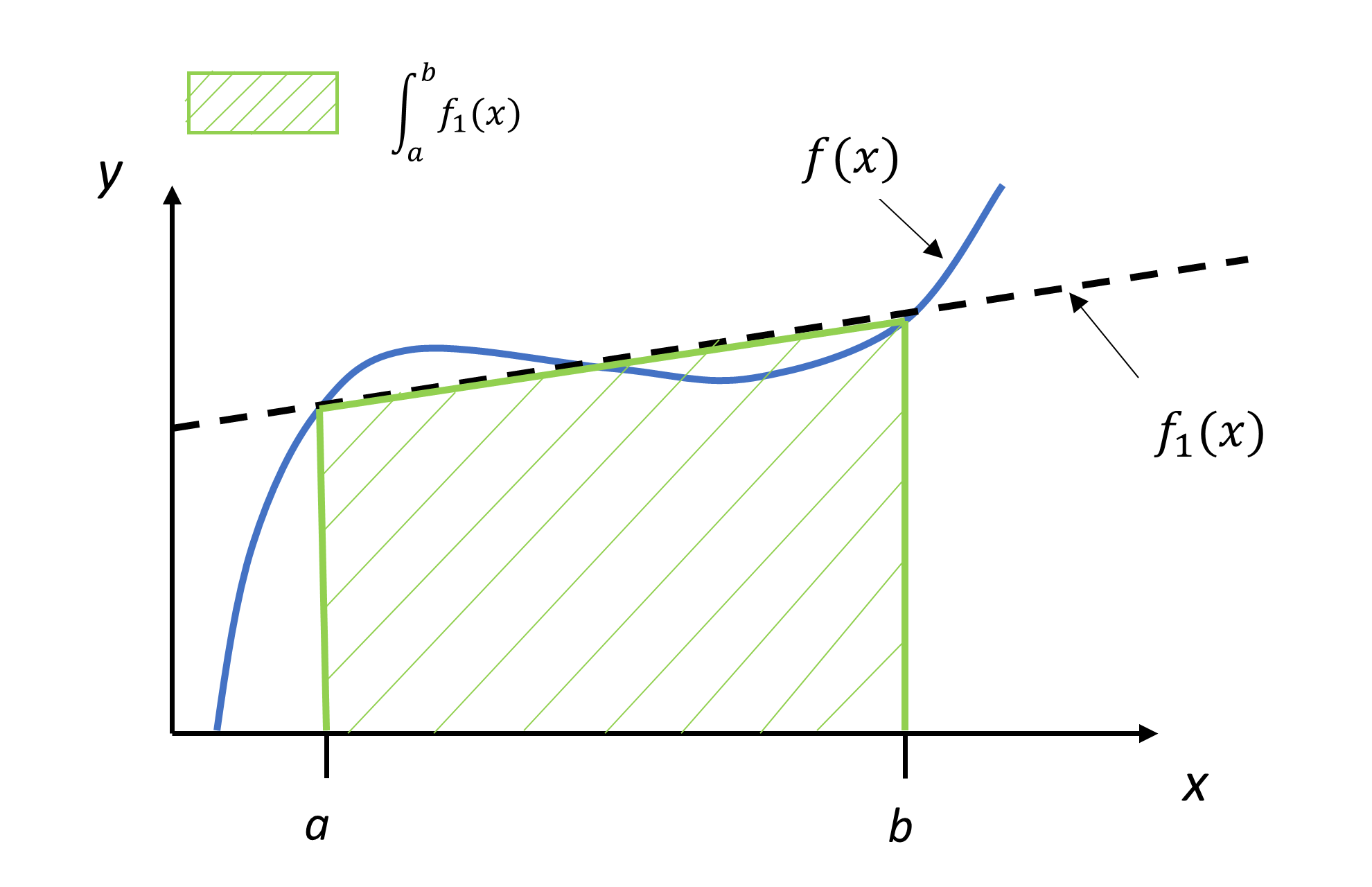
Approximating the integrand \(f(x)\) by a first-order polynomial \(f_{1}(x)\), that is, \(f_{1}(x) = a_{0} + a_{1}x\),
\[\begin{split} \int_{a}^{b} f(x) \ dx &\approx \int_{a}^{b} f_{1}(x) \ dx\\ &= \int_{a}^{b} (a_{0} + a_{1}x) \ dx\\ &= a_{0}(b - a) + a_{1}\left( \frac{b^{2} - a^{2}}{2} \right)\;\;\;\;\;\;\;\;\;\;\;\; (\PageIndex{1.5}) \end{split}\]
But what are \(a_{0}\) and \(a_{1}\)? Now if one chooses \((a,f(a))\) and \((b,f(b))\) as the two points to approximate \(f(x)\) by a straight line from \(a\) to \(b\),
\[\begin{split} f(a) &= f_{1}(a) = a_{0} + a_{1}a\\ f(b) &= f_{1}(b) = a_{0} + a_{1}b\;\;\;\;\;\;\;\;\;\;\;\; (\PageIndex{1.6a,b})\end{split}\]
Solving Equations \((\PageIndex{1.6a})\) and \((\PageIndex{1.6b})\) for \(a_{0}\) and \(a_{1}\), we get
\[a_{1} = \frac{f(b) - f(a)}{b - a} \nonumber\]
\[a_{0} = \frac{f(a)b - f(b)a}{b - a}\;\;\;\;\;\;\;\;\;\;\;\; (\PageIndex{1.7a,b}) \nonumber\]
Substituting values of \(a_0\) and \(a_1\) from Equations \((\PageIndex{1.7a})\) and \((\PageIndex{1.7b})\) in Equation \((\PageIndex{1.5})\) gives
\[\begin{split} \int_{a}^{b} f(x) \ dx &\approx \frac{f(a)b - f(b)a}{b - a}(b - a) + \frac{f(b) - f(a)}{b - a}\frac{b^{2} - a^{2}}{2}\\ &= (b - a)\left\lbrack \frac{f(a) + f(b)}{2} \right\rbrack\;\;\;\;\;\;\;\;\;\;\;\; (\PageIndex{1.8}) \end{split}\]
Note that the trapezoidal rule can be interpreted as the width of the interval \([a,b]\) multiplied to an approximate average value of the function. Recall the definition of the mean of the function \(\overline{f}\) of a function \(f\) in an interval \(\lbrack a,b\rbrack\) is given by \[\displaystyle \overline{f} = \frac{1}{b - a}\int_{a}^{b}f(x) \ dx\;\;\;\;\;\;\;\;\;\;\;\; (\PageIndex{1.9}) \nonumber\]
The following integral is given
\[\int_{0.1}^{1.3} 5xe^{- 2x} \ dx \nonumber\]
a) Use the trapezoidal rule to estimate the value of the integral.
b) Find the true error, \(E_{t}\), for part (a).
c) Find the absolute relative true error, \(\left| \varepsilon_{t} \right|\), for part (a).
Solution
a) From Equation \((\PageIndex{1.8}\), which is repeated here,
\[\int_{b}^{a} f(x) \ dx \approx \frac{(b - a)}{2} \left[ f(a) + f(b) \right] \nonumber\]
where
\[a = 0.1 \nonumber\]
\[b = 1.3 \nonumber\]
Then
\[\begin{split}\int_{0.1}^{1.3} f(x) dx &\approx \frac{(1.3 - 0.1)}{2}\left\lbrack f(0.1) + f(1.3) \right\rbrack\\ &= 0.6\left\lbrack f(0.1) + f(1.3) \right\rbrack\\ &= 0.6\lbrack 5(0.1)e^{- 2(0.1)} + 5(1.3)e^{- 2(1.3)}\rbrack\\ &= 0.6(0.4094 + 0.4828)\\ &= 0.5353 \end{split}\]
b) The true error is
\[\begin{split} E_{t} &=\ \text{True Value} - \text{Approximate Value}\\ &= 0.8939 - 0.5353\\ &= 0.3586 \end{split}\]
c) The absolute relative true error, \(\left| \varepsilon_{t} \right|\), would then be
\[\begin{split} \left| \varepsilon_{t} \right| &= \left| \frac{\text{True Error}}{\text{True Value}} \right| \times 100\\ &= \left| \frac{0.3586}{0.8939} \right| \times 100\\ &= 40.12\% \end{split}\]
The vertical distance covered by a rocket from \(t = 8\) to \(t = 30\) seconds is given by
\[x = \int_{8}^{30} \left( 2000\ln\left\lbrack \frac{140000}{140000 - 2100t} \right\rbrack - 9.8t \right) \ dt \nonumber\]
a) Use the trapezoidal rule to find the distance covered for \(t = 8\) to \(t = 30\) seconds.
b) Find the true error, \(E_{t}\) for part (a).
c) Find the absolute relative true error for part (a).
Solution
a) \[I \approx (b - a)\left\lbrack \frac{f(a) + f(b)}{2} \right\rbrack, \nonumber\] where
\[a = 8 \nonumber\]
\[b = 30 \nonumber\]
\[f(t) = 2000\ln\left\lbrack \frac{140000}{140000 - 2100t} \right\rbrack - 9.8t \nonumber\]
\[\begin{split} f(8) &= 2000\ln\left\lbrack \frac{140000}{140000 - 2100(8)} \right\rbrack - 9.8(8)\\ &= 177.27\ \text{m/s}\end{split}\]
\[\begin{split} f(30) &= 2000\ln\left\lbrack \frac{140000}{140000 - 2100(30)} \right\rbrack - 9.8(30)\\ &= 901.67\ \text{m/s}\end{split}\]
\[\begin{split} I &\approx (30 - 8)\left\lbrack \frac{177.27 + 901.67}{2} \right\rbrack\\ &= 11868\ \text{m}\end{split}\]
b) The exact value of the above integral is
\[\begin{split} x &= \int_{8}^{30} \left( 2000\ln\left\lbrack \frac{140000}{140000 - 2100t} \right\rbrack - 9.8t \right) \ dt\\ &= 11061\ \text{m}\end{split}\]
so the true error is
\[\begin{split} E_{t} &= \text{True Value} - \text{Approximate Value}\\ &= 11061 - 11868\\ &= - 807\ \text{m}\end{split}\]
c) The absolute relative true error, \(\left| \epsilon_{t} \right|\), would then be
\[\begin{split} \left| \epsilon_{t} \right| &= \left| \frac{\text{True Error}}{\text{True Value}} \right| \times 100\\ &= \left| \frac{11061 - 11868}{11061} \right| \times 100\\ &= 7.2958\% \end{split}\]
Audiovisual Lecture
Title: Single Application Trapezoidal Example
Summary: Learn the trapezoidal rule of integration through a simple example.
Appendix 1
This appendix shows other methods of deriving the trapezoidal rule of integration. The method of undetermined coefficients is significant to learn as it forms the basis of the Gauss quadrature rule.
Method 2: Derived from Calculus Using Newton’s divided difference polynomial
\(f_{1}(x)\) can also be approximated by using Newton’s divided difference polynomial as
\[f_{1}(x) = f(a) + \frac{f(b) - f(a)}{b - a}(x - a)\;\;\;\;\;\;\;\;\;\;\;\; (\PageIndex{A1.1}) \nonumber\]
Hence
\[\begin{split} \int_{a}^{b} f(x) \ dx &\approx \int_{a}^{b} f_{1}(x) \ dx\\ &= \int_{a}^{b} \left\lbrack f(a) + \frac{f(b) - f(a)}{b - a}(x - a) \right\rbrack \ dx\\ &= \left\lbrack f(a)x + \frac{f(b) - f(a)}{b - a}\left( \frac{x^{2}}{2} - {ax} \right) \right\rbrack_{a}^{b}\\ &= f(a)b - f(a)a + \left( \frac{f(b) - f(a)}{b - a} \right)\left( \frac{b^{2}}{2} - {ab} - \frac{a^{2}}{2} + a^{2} \right)\\ &= f(a)b - f(a)a + \left( \frac{f(b) - f(a)}{b - a} \right)\left( \frac{b^{2}}{2} - ab + \frac{a^{2}}{2} \right)\\ &= f(a)b - f(a)a + \left( \frac{f(b) - f(a)}{b - a} \right)\frac{1}{2}\left( b - a \right)^{2}\\ &= f(a)b - f(a)a + \frac{1}{2}\left( f(b) - f(a) \right)\left( b - a \right)\\ &= f(a)b - f(a)a + \frac{1}{2}f(b)b - \frac{1}{2}f(b)a - \frac{1}{2}f(a)b + \frac{1}{2}f(a)a\\ &= \frac{1}{2}f(a)b - \frac{1}{2}f(a)a + \frac{1}{2}f(b)b - \frac{1}{2}f(b)a\\ &= (b - a)\left\lbrack \frac{f(a) + f(b)}{2} \right\rbrack\;\;\;\;\;\;\;\;\;\;\;\; (\PageIndex{A1.2}) \end{split}\]
This gives the same result as Equation \((\PageIndex{1.8})\) because \(f_1(x)\) is just a different form of writing the same first-order polynomial.
Method 3: Derived from Geometry
The trapezoidal rule can also be derived from geometry. Look at Figure \(\PageIndex{1.2}\). The area under the curve \(f_{1}(x)\) is the area of a trapezoid. The integral
\[\begin{split} \int_{a}^{b}{f(x)dx} &\approx \text{Area of trapezoid}\\ &= \frac{1}{2} \text{(Sum of the length of parallel sides)}\\ & \ \ \ \ \ \ \ \ \ \ \ \times \text{(Perpendicular distance between the parallel sides)}\\ &= \frac{1}{2}\left( f(b) + f(a) \right)(b - a)\\ &= (b - a)\left\lbrack \frac{f(a) + f(b)}{2} \right\rbrack\;\;\;\;\;\;\;\;\;\;\;\; (\PageIndex{A1.3}) \end{split}\]
Audiovisual Lecture
Title: Single-Application Trapezoidal Rule Derivation
Summary: Learn how to derive the trapezoidal rule of integration.
Method 4: Derived from Method of Coefficients
Choose the integral \(\displaystyle \int_{a}^{b} f(x) \ dx\) approximated as follows.
\[\int_{a}^{b} f(x) \ dx \approx c_{1}f(a) + c_{2}f(b)\;\;\;\;\;\;\;\;\;\;\;\; (\PageIndex{A1.4}) \nonumber\]
The coefficients \(c_{1}\) and \(c_{2}\) are undetermined. We will find these coefficients such that the right-hand side is exact for integrals of a straight line \(a_{0} + a_{1}x\).
So from exact integration
\[\begin{split} \int_{a}^{b} \left( a_{0} + a_{1}x \right) \ dx &= \left\lbrack a_{0}x + a_{1}\frac{x^{2}}{2} \right\rbrack_{a}^{b}\\ &= a_{0}\left( b - a \right) + a_{1}\left( \frac{b^{2} - a^{2}}{2} \right)\;\;\;\;\;\;\;\;\;\;\;\; (\PageIndex{A1.5}) \end{split}\]
But we want the right-hand side formula to give the same result as Equation \((\PageIndex{A1.5})\) for \(f(x) = a_{0} + a_{1}x\) which is
\[\begin{split} c_{1}f(a) + c_{2}f(b) &= c_{1}(a_{0} + a_{1}b) + c_{2}(a_{0} + a_{1}b) \\ &= a_{0}\left( c_{1} + c_{2} \right) + a_{1}\left ( c_{1}a + c_{2}b \right)\;\;\;\;\;\;\;\;\;\;\;\; (\PageIndex{A1.6}) \end{split}\]
Hence from Equations \((\PageIndex{A1.5})\) and \((\PageIndex{A1.6})\),
\[a_{0}\left( b - a \right) + a_{1}\left( \frac{b^{2} - a^{2}}{2} \right) = a_{0}\left( c_{1} + c_{2} \right) + a _{1}\left( c_{1}a + c_{2}b \right)\;\;\;\;\;\;\;\;\;\;\;\; (\PageIndex{A1.7}) \nonumber\]
Since \(a_{0}\) and \(a_{1}\) are arbitrary constants for the chosen general straight line, the coefficients of \(a_{0}\) and \(a_{1}\) need to be equal. That gives
\[c_{1} + c_{2} = b - a\;\;\;\;\;\;\;\;\;\;\;\; (\PageIndex{A1.8a}) \nonumber\]
\[c_{1}a + c_{2}b = \frac{b^{2} - a^{2}}{2}\;\;\;\;\;\;\;\;\;\;\;\; (\PageIndex{A1.8b}) \nonumber\]
Multiplying Equation \((\PageIndex{A1.8a})\) by \(a\) and subtracting from Equation \((\PageIndex{A1.8b})\) gives
\[c_{2} = \frac{b - a}{2}\;\;\;\;\;\;\;\;\;\;\;\; (\PageIndex{A1.9a}) \nonumber\]
Substituting the value of \(c_{2}\) from Equation \((\PageIndex{A1.9a})\) in Equation \((\PageIndex{A1.8a})\) gives
\[c_{1} = \frac{b - a}{2}\;\;\;\;\;\;\;\;\;\;\;\; (\PageIndex{A1.9b}) \nonumber\]
Therefore, from Equation \((\PageIndex{A1.4})\), \((\PageIndex{A1.9a})\), and \((\PageIndex{A1.9b})\),
\[\begin{split} \int_{a}^{b}f(x) \ dx &\approx c_{1}f(a) + c_{2}f(b)\\ &= \frac{b - a}{2}f(a) + \frac{b - a}{2}f(b)\;\;\;\;\;\;\;\;\;\;\;\; (\PageIndex{A1.10}) \end{split}\]
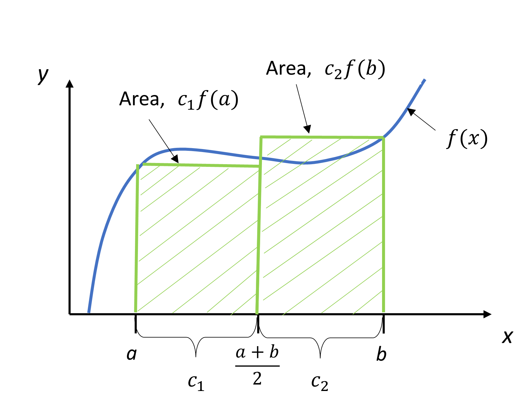
The interpretation is that \(f(x)\) is evaluated at points \(a\) and \(b\), and each function evaluation is given a weight of \(\displaystyle \frac{b - a}{2}\). Geometrically, Equation \((\PageIndex{1.8})\) is looked at as the area of a trapezoid, while Equation \((\PageIndex{A1.10})\) is viewed as the sum of the area of two rectangles, as shown in Figure \(\PageIndex{1.3}\).
Lesson 2: Composite Trapezoidal Rule
Learning Objectives
After successful completion of this lesson, you should be able to:
1) derive the composite (also called multiple-segment) trapezoidal rule of integration,
2) use the composite (also called multiple-segment) trapezoidal rule of integration to solve problems
Introduction
A single segment trapezoidal rule seldom gives you acceptable results for an integral. Instead for higher accuracy and its control, we can use the composite (also called multiple-segment) trapezoidal rule where the integral is broken into segments, and the single-segment trapezoidal rule is applied over each segment.
Derivation
Divide \((b - a)\) into \(n\) equal segments, as shown in Figure \(\PageIndex{2.1}\). Then the width of each segment is
\[h = \frac{b - a}{n}\;\;\;\;\;\;\;\;\;\;\;\; (\PageIndex{2.1}) \nonumber\]
The integral \(I\) can be broken into \(n\) integrals as
\[\begin{split} I &= \int_{a}^{b} f(x) \ dx\\ &= \int_{a}^{a + h} f(x) \ dx + \int_{a + h}^{a + 2h} f(x) \ dx + ... + \int_{a + (n - 2)h}^{a + (n - 1)h} f(x) \ dx + \int_{a + (n - 1)h}^{b} f(x) \ dx\;\;\;\;\;\;\;\;\;\;\;\; (\PageIndex{2.2}) \end{split}\]
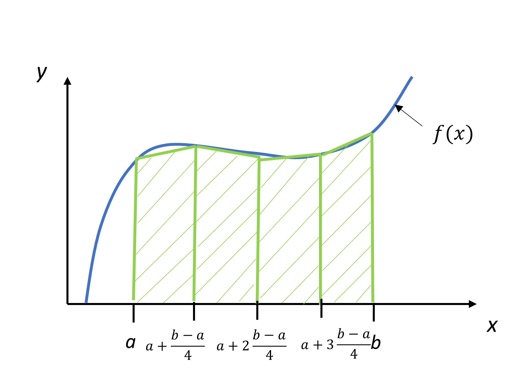
Applying single-segment trapezoidal rule on Equation \((\PageIndex{2.2})\) on each segment gives
\[\begin{split} \int_{a}^{b} f(x) \ dx &\approx \left\lbrack (a + h) - a \right\rbrack\left\lbrack \frac{f(a) + f(a + h)}{2} \right\rbrack\\ & + \left\lbrack (a + 2h) - (a + h) \right\rbrack\left\lbrack \frac{f(a + h) + f(a + 2h)}{2} \right\rbrack\\ &\ +............... \\ & + \left[\left(a+(n-1)h\right)-\left(a+(n-2)h\right)\right]\left\lbrack \frac{f(a + (n - 2)h) + f(a + (n - 1)h)}{2} \right\rbrack\\ &+ \left\lbrack b - \left( a + (n - 1)h \right) \right\rbrack\left\lbrack \frac{f(a + (n - 1)h) + f(b)}{2} \right\rbrack\\ \\ &= h\left\lbrack \frac{f(a) + f(a + h)}{2} \right\rbrack + h\left\lbrack \frac{f(a + h) + f(a + 2h)}{2} \right\rbrack\\ & \ + ............... \\ &+ h\left\lbrack \frac{f(a + (n - 2)h) + f(a + (n - 1)h)}{2} \right\rbrack\\ &+ h\left\lbrack \frac{f(a + (n - 1)h) + f(b)}{2} \right\rbrack\\ \\ &= h\left\lbrack \frac{f(a) + 2f(a + h) + 2f(a + 2h) + ... + 2f(a + (n - 1)h) + f(b)}{2} \right\rbrack\\ &= \frac{h}{2}\left\lbrack f(a) + 2\left\{ \sum_{i = 1}^{n - 1}{f(a + {ih})} \right\} + f(b) \right\rbrack\\ &= \frac{b - a}{2n}\left\lbrack f(a) + 2\left\{ \sum_{i = 1}^{n - 1}{f(a + {ih})} \right\} + f(b) \right\rbrack\;\;\;\;\;\;\;\;\;\;\;\; (\PageIndex{2.3}) \end{split}\]
Audiovisual Lecture
Title: Derivation of Composite Trapezoidal Rule of Integration
Summary: Learn the derivation of and motivation behind the composite trapezoidal rule of integration.
The following integral is given:
\[\int_{0.1}^{1.3} 5xe^{- 2x} \ dx \nonumber\]
a) Use the composite trapezoidal rule to estimate the value of this integral. Use three segments.
b) Find the true error \(E_{t}\) for part (a).
c) Find the absolute relative true error \(\left| \varepsilon_{t} \right|\) for part (a).
Solution
a) The solution using the composite trapezoidal rule with 3 segments is applied as follows.
\[I \approx \frac{b - a}{2n}\left\lbrack f(a) + 2\sum_{i = 1}^{n - 1}{f(a + {ih})} + f(b) \right\rbrack \nonumber\]
\[n = 3 \nonumber\]
\[a = 0.1 \nonumber\]
\[b = 1.3 \nonumber\]
\[\begin{split} h &= \frac{b - a}{n}\\ &= \frac{1.3 - 0.1}{3}\\ &= 0.4 \end{split}\]
From Equation \((\PageIndex{2.3})\),
\[\begin{split} I &\approx \frac{1.3 - 0.1}{6}\left\lbrack f(0.1) + 2\sum_{i = 1}^{3 - 1}{f(0.1 + 0.4i)} + f(1.3) \right\rbrack\\ I &\approx \frac{1.3 - 0.1}{6}\left\lbrack f(0.1) + 2\sum_{i = 1}^{2}{f(0.1 + 0.4i)} + f(1.3) \right\rbrack\\ &= 0.2\lbrack f(0.1) + 2f(0.5) + 2f(0.9) + f(1.3)\rbrack\\ &= 0.2[5 \times 0.1 \times e^{- 2(0.1)}+2(5 \times 0.5 \times e^{- 2(0.5)})+2(5 \times 0.9 \times e^{- 2(0.9)}) + 5 \times 1.3 \times e^{- 2(1.3)}\rbrack\\ &= 0.84385 \end{split}\]
b) The exact value of the above integral can be found by integration by parts and is
\[\int_{0.1}^{1.3} 5xe^{- 2x} \ dx = 0.89387 \nonumber\]
So the true error is
\[\begin{split} E_{t} &= \text{True Value} - \text{Approximate Value}\\ &= 0.89387 - 0.84385\\ &= 0.05002 \end{split}\]
c) The absolute relative true error is
\[\displaystyle \begin{split}\left| \varepsilon_{t} \right| &= \left| \frac{\text{True Error}}{\text{True Value}} \right| \times 100\\ &= \left| \frac{0.05002}{0.89387} \right| \times 100\\ &= 5.5959\% \end{split}\]
The vertical distance covered by a rocket from \(t = 8\) to \(t = 30\) seconds is given by
\[x = \int_{8}^{30} \left( 2000\ln\left\lbrack \frac{140000}{140000 - 2100t} \right\rbrack - 9.8t \right) \ dt \nonumber\]
a) Use the composite trapezoidal rule to find the distance covered from \(t = 8\) to \(t = 30\) seconds. Use two segments.
b) Find the true error, \(E_{t}\), for part (a).
c) Find the absolute relative true error for part (a).
Solution
a) The solution using the composite trapezoidal rule with 2-segments is
\[I \approx \frac{b - a}{2n}\left\lbrack f(a) + 2\left\{ \sum_{i = 1}^{n - 1}{f(a + ih)} \right\} + f(b) \right\rbrack \nonumber\]
\[n = 2 \nonumber\]
\[a = 8 \nonumber\]
\[b = 30 \nonumber\]
\[\begin{split} h &= \frac{b - a}{n}\\ &= \frac{30 - 8}{2}\\ &= 11 \end{split} \nonumber\]
\[\begin{split} I &\approx \frac{30 - 8}{2(2)}\left\lbrack f(8) + 2\left\{ \sum_{i = 1}^{2 - 1}{f(8 + 11i)} \right\} + f(30) \right\rbrack\\ &= \frac{22}{4}\left\lbrack f(8) + 2f(19) + f(30) \right\rbrack\\ &= \frac{22}{4}\left\lbrack 177.27 + 2(484.75) + 901.67 \right\rbrack\\ &= 11266\ \text{m}\end{split}\]
b) The exact value of the above integral is
\[\begin{split} x &= \int_{8}^{30}{\left( 2000\ln\left\lbrack \frac{140000}{140000 - 2100t} \right\rbrack - 9.8t \right){dt}}\\ &= 11061\ \text{m}\end{split}\]
So the true error is
\[\begin{split} E_{t} &= \text{True Value} -\text{Approximate Value}\\ &= 11061 - 11266\\ &= - 205\ \text{m}\end{split}\]
c) The absolute relative true error,\(\left| \epsilon_{t} \right|\), would then be
\[\begin{split} \left| \epsilon_{t} \right| &= \left| \frac{\text{True Error}}{\text{True Value}} \right| \times 100\\ &= \left| \frac{11061 - 11266}{11061} \right| \times 100\\ &= 1.8537\% \end{split}\]
| \(n\) | \(\text{Approximate Value}\) | \(E_{t}\) | \(\left| \epsilon_{t } \right|\%\) | \(\left| \epsilon_{a } \right|\%\) |
|---|---|---|---|---|
| \(1\) | \(11868\) | \(-807\) | \(7.296\) | \(---\) |
| \(2\) | \(11266\) | \(-205\) | \(1.853\) | \(5.343\) |
| \(3\) | \(11153\) | \(-91.4\) | \(0.8265\) | \(1.019\) |
| \(4\) | \(11113\) | \(-51.5\) | \(0.4655\) | \(0.3594\) |
| \(5\) | \(11094\) | \(-33.0\) | \(0.2981\) | \(0.1669\) |
| \(6\) | \(11084\) | \(-22.9\) | \(0.2070\) | \(0.09082\) |
| \(7\) | \(11078\) | \(-16.8\) | \(0.1521\) | \(0.05482\) |
| \(8\) | \(11074\) | \(-12.9\) | \(0.1165\) | \(0.03560\) |
Audiovisual Lecture
Title: Example for Composite Trapezoidal Rule of Integration
Summary: Learn how composite trapezoidal rule of integration is used via example.
Error in Composite Trapezoidal Rule
Without proof, the true error for a single-segment Trapezoidal rule for \(\displaystyle \int_{a}^{b} f(x) \ dx\) is given by
\[E_{t} = - \frac{(b - a)^{3}}{12}f^{\prime\prime}(\zeta),\ a < \zeta < b\;\;\;\;\;\;\;\;\;\;\;\; (\PageIndex{2.4}) \nonumber\]
where
\[\zeta\ \text{ is some point in}\ \left\lbrack a,b \right\rbrack. \nonumber\]
What is the error then in the composite trapezoidal rule for \(\int_{a}^{b} f(x) \ dx\)?
It is given by
\[E_{t} \approx - \frac{(b - a)^{3}}{12n^{2}}\overline{f^{\prime\prime}}\;\;\;\;\;\;\;\;\;\;\;\; (\PageIndex{2.5}) \nonumber\]
where
\[\begin{split} \overline{f^{\prime\prime}} =\ &\text{some approximate average value of the second derivative}\\ &\text{of the function in}\ \left\lbrack a,b \right\rbrack.\end{split}\]
\[n = \text{number of segments.} \nonumber\]
Recall that the width of each segment is
\[h=\frac{b-a}{n} \nonumber\]
Appendix 2
The appendix gives you two more examples for showing the application of the composite trapezoidal rule.
Use the composite trapezoidal rule to find the area under the curve
\[f(x) = \frac{300x}{1 + e^{x}} \nonumber\]
from \(x = 0\) to \(x = 10\). Use 2 segments.
Solution
Using two segments, we get
\[h = \frac{10 - 0}{2} = 5 \nonumber\]
\[f(0) = \frac{300(0)}{1 + e^{0}} = 0 \nonumber\]
\[f(5) = \frac{300(5)}{1 + e^{5}} = 10.039 \nonumber\]
\[f(10) = \frac{300(10)}{1 + e^{10}} = 0.136 \nonumber\]
From Equation \((\PageIndex{2.3})\)
\[\begin{split} I &\approx \frac{b - a}{2n}\left\lbrack f(a) + 2\left\{ \sum_{i = 1}^{n - 1}{f(a + ih)} \right\} + f(b) \right\rbrack\\ &= \frac{10 - 0}{2(2)}\left\lbrack f(0) + 2\left\{ \sum_{i = 1}^{2 - 1}{f(0 + 5)} \right\} + f(10) \right\rbrack\\ &= \frac{10}{4}\left\lbrack f(0) + 2f(5) + f(10) \right\rbrack\\ &= \frac{10}{4}\left\lbrack 0 + 2(10.039) + 0.136 \right\rbrack\\ &= 50.537 \end{split}\]
So what is the true value of this integral?
\[\int_{0}^{10} \frac{300x}{1 + e^{x}} \ dx = 246.59 \nonumber\]
The absolute relative true error is
\[\begin{split} \left| \epsilon_{t} \right| &= \left| \frac{246.59 - 50.535}{246.59} \right| \times 100\\ &= 79.506\% \end{split}\]
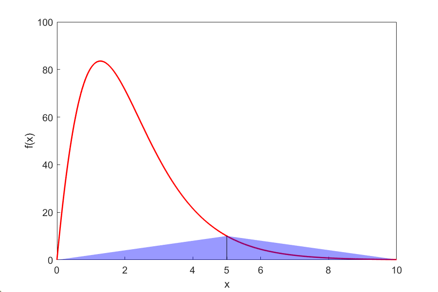
Why is the true value different from the approximate values? Just take a look at Figure \(\PageIndex{2.2}\). As you can see, the area under the “trapezoids” (yeah, they really look like triangles now) covers a small portion of the area under the curve. As we add more segments, the approximated value quickly approaches the true value.
| \(n\) | \(\text{Approximate Value}\) | \(E_{t}\) | \(\left| \epsilon_{t} \right|\) |
|---|---|---|---|
| \(1\) | \(0.681\) | \(245.91\) | \(99.724\%\) |
| \(2\) | \(50.535\) | \(196.05\) | \(79.505\%\) |
| \(4\) | \(170.61\) | \(75.978\) | \(30.812\%\) |
| \(8\) | \(227.04\) | \(19.546\) | \(7.927\%\) |
| \(16\) | \(241.70\) | \(4.887\) | \(1.982\%\) |
| \(32\) | \(245.37\) | \(1.222\) | \(0.495\%\) |
| \(64\) | \(246.28\) | \(0.305\) | \(0.124\%\) |
Use the composite trapezoidal rule to find
\[I = \int_{0}^{2} \frac{1}{\sqrt{x}} \ dx \nonumber\]
Solution
We cannot use the trapezoidal rule for this integral, as the value of the integrand at \(x = 0\) is infinite. However, it is known that discontinuities in a curve do not change the area under it. We can assume any value for the function at \(x = 0\). The algorithm to define the function so that we can use the composite trapezoidal rule is given below.
\[\text{Function}\ f(x) \nonumber\]
\[\text{If}\ x = 0\ \text{Then}\ f = 0 \nonumber\]
\[\text{If}\ x \neq 0\ \text{Then}\ f = x^{( - 0.5)} \nonumber\]
\[\text{End Function} \nonumber\]
Basically, we are just assigning the function a value of zero at \(x = 0\). Everywhere else, the function is continuous. This assumption means the true value of our integral is just that—true. Let’s see what happens using the composite trapezoidal rule.
Using two segments, we get
\[h = \frac{2 - 0}{2} = 1 \nonumber\]
\[f(0) = 0 \nonumber\]
\[f(1) = \frac{1}{\sqrt{1}} = 1 \nonumber\]
\[f(2) = \frac{1}{\sqrt{2}} = 0.70711 \nonumber\]
\[\begin{split} I &\approx \frac{b - a}{2n}\left\lbrack f(a) + 2\left\{ \sum_{i = 1}^{n - 1}{f(a + ih)} \right\} + f(b) \right\rbrack\\ &= \frac{2 - 0}{2(2)}\left\lbrack f(0) + 2\left\{ \sum_{i = 1}^{2 - 1}{f(0 + 1)} \right\} + f(2) \right\rbrack\\ &= \frac{2}{4}\left\lbrack f(0) + 2f(1) + f(2) \right\rbrack\\ &= \frac{2}{4}\left\lbrack 0 + 2(1) + 0.70711 \right\rbrack\\ &= 1.3536 \end{split}\]
So what is the true value of this integral?
\[\int_{0}^{2} \frac{1}{\sqrt{x}} \ dx = 2.8284 \nonumber\]
thus making the absolute relative true error
\[\begin{split} \left| \epsilon_{t} \right| &= \left| \frac{2.8284 - 1.3536}{2.8284} \right| \times 100\\ &= 52.145\% \end{split}\]
Table \(\PageIndex{A2.2}\) shows how the approximate value converges to the true value as the number of segments is increased.
| \(n\) | \(\text{Approximate Value}\) | \(E_{t}\) | \(\left|\epsilon_t\right|\) |
|---|---|---|---|
| \(2\) | \(1.354\) | \(1.474\) | \(52.14\%\) |
| \(4\) | \(1.792\) | \(1.036\) | \(36.64\%\) |
| \(8\) | \(2.097\) | \(0.731\) | \(25.85\%\) |
| \(16\) | \(2.312\) | \(0.516\) | \(18.26\%\) |
| \(32\) | \(2.463\) | \(0.365\) | \(12.91\%\) |
| \(64\) | \(2.570\) | \(0.258\) | \(9.128\%\) |
| \(128\) | \(2.646\) | \(0.182\) | \(6.454\%\) |
| \(256\) | \(2.699\) | \(0.129\) | \(4.564\%\) |
| \(512\) | \(2.737\) | \(0.091\) | \(3.227\%\) |
| \(1024\) | \(2.764\) | \(0.064\) | \(2.282\%\) |
| \(2048\) | \(2.783\) | \(0.045\) | \(1.613\%\) |
| \(4096\) | \(2.796\) | \(0.032\) | \(1.141\%\) |
Lesson 3: Error Analysis of Trapezoidal Rule
Learning Objective
After successful completion of this lesson, you should be able to:
1) derive the formula for the true error in the composite (also called multiple-segment) trapezoidal rule of integration.
Error in Composite Trapezoidal Rule
The true error for a single segment trapezoidal rule is given by
\[E_{t} = - \frac{(b - a)^{3}}{12}f^{\prime\prime}(\zeta),\ a < \zeta < b\;\;\;\;\;\;\;\;\;\;\;\; (\PageIndex{3.1}) \nonumber\]
where \[\zeta\ \text{is some point in}\ \left\lbrack a,b \right\rbrack. \nonumber\]
What is the error then in the composite trapezoidal rule? It is the sum of the errors from each of the \(n\) segments. The error in each segment is that of the single segment trapezoidal rule. The error in each segment is
\[\begin{split} E_{1} &= - \frac{\left\lbrack (a + h) - a \right\rbrack^{3}}{12}f^{\prime\prime} (\zeta_{1}),a < \zeta_{1} < a + h\\ &= - \frac{h^{3}}{12}f^{\prime\prime} (\zeta_{1})\end{split} \nonumber\] \[\begin{split}E_{2} &= - \frac{\left\lbrack (a + 2h) - (a + h) \right\rbrack^{3}}{12}f^{\prime\prime} (\zeta_{2}),a + h < \zeta_{2} < a + 2h\\ &= - \frac{h^{3}}{12}f^{\prime\prime} (\zeta_{2})\end{split} \nonumber\] \[\vdots \nonumber\] \[\begin{split}E_{i} &= - \frac{\left\lbrack (a + ih) - (a + (i - 1)h) \right\rbrack^{3}}{12}f^{\prime\prime} (\zeta_{i}),a + (i - 1)h < \zeta_{i} < a + ih\\ &= - \frac{h^{3}}{12}f^{\prime\prime} (\zeta_{i})\\ \end{split} \nonumber\] \[\vdots \nonumber\]
\[\begin{split} E_{n - 1} &= - \frac{\left\lbrack \left\{ a + (n - 1)h \right\} - \left\{ a + (n - 2)h \right\} \right\rbrack^{3}}{12}f^{\prime\prime} (\zeta_{n - 1}),a + (n - 2)h < \zeta_{n - 1} < a + (n - 1)h\\ &= - \frac{h^{3}}{12}f^{\prime\prime} (\zeta_{n - 1})\end{split} \nonumber\] \[\begin{split}E_{n} &= - \frac{\left\lbrack b - \left\{ a + (n - 1)h \right\} \right\rbrack^{3}}{12}f^{\prime\prime} (\zeta_{n}),a + (n - 1)h < \zeta_{n} < b\\ &= - \frac{h^{3}}{12}f^{\prime\prime} (\zeta_{n}) \end{split} \nonumber\]
Hence the total error in the composite trapezoidal rule is
\[\begin{split} E_{t} &= \sum_{i = 1}^{n}E_{i} \\&=-\frac{h^3}{12}f^{\prime\prime}(\zeta_1)- \frac{h^3}{12}f^{\prime\prime}(\zeta_2)-\ldots-\frac{h^3}{12}f^{\prime\prime}(\zeta_n) \\ &= - \frac{h^{3}}{12}\sum_{i = 1}^{n}{f^{\prime\prime} (\zeta_i})\end{split}\]
Since \(h=\displaystyle \frac{b-a}{n}\),
\[\begin{split} E_t &= - \frac{(b - a)^{3}}{12n^{3}}\sum_{i = 1}^{n}{f^{\prime\prime} (\zeta_{i})}\\ &= - \frac{(b - a)^{3}}{12n^{2}}\frac{\displaystyle \sum_{i = 1}^{n}{f^{\prime\prime} (\zeta_{i})}}{n}\end{split}\]
The term \(\displaystyle \frac{\displaystyle \sum_{i = 1}^{n}{f^{\prime\prime} (\zeta_{i})}}{n}\) is an approximate average value of the second derivative\(\ f^{\prime\prime} (x),a < x < b\).
Hence
\[E_{t} \approx - \frac{(b - a)^{3}}{12n^{2}}\ \overline{f^{\prime\prime}}\;\;\;\;\;\;\;\;\;\;\;\; (\PageIndex{3.2}) \nonumber\]
In Table \(\PageIndex{3.1}\), the approximate value of the integral
\[\int_{8}^{30} \left( 2000\ln\left\lbrack \frac{140000}{140000 - 2100t} \right\rbrack - 9.8t \right) \ dt \nonumber\]
is given as a function of the number of segments in a composite trapezoidal rule. You can visualize that as the number of segments is doubled, the true error gets approximately quartered.
| \(\text{n}\) | \(\text{Approximate Value}\) | \(E_{t}\) | \(\left|\epsilon_{t }\right|\%\) | \(\left|\epsilon_{a }\right|\%\) |
|---|---|---|---|---|
| \(2\) | \(11266\) | \(-205\) | \(1.853\) | \(5.343\) |
| \(4\) | \(11113\) | \(-52\) | \(0.4701\) | \(0.3594\) |
| \(8\) | \(11074\) | \(-13\) | \(0.1175\) | \(0.03560\) |
| \(16\) | \(11065\) | \(-4\) | \(0.03616\) | \(0.00401\) |
For example, for the composite trapezoidal rule with 2 segments, the true error is \(-205\), and a quarter of that error is \(-51.25\). That is close to the true error of \(-52\) for the composite trapezoidal rule with 4 segments.
Can you answer the question, why is the true error not exactly \(-51.25\)? How does this information help us in numerical integration? You will find out that this forms the basis of Richardson’s extrapolation formula for integration based on the trapezoidal rule, where we use the argument that true error gets approximately quartered when the number of segments is doubled. Richardson’s extrapolation formula based on the trapezoidal rule is computationally more efficient than using the composite trapezoidal rule by itself.
Audiovisual Lecture
Title: Composite Trapezoidal Rule Error: Derivation
Summary: This video discusses how to derive the error formula for the composite trapezoidal rule.
Audiovisual Lecture
Title: Composite Trapezoidal Rule Error: Example
Summary: After watching this video, via an example, you will be able to use the formula for the true error in the composite trapezoidal rule. You will see how the true error is approximately inversely proportional to the square of the number of segments.
Richardson’s Extrapolation Formula for Trapezoidal Rule
From Equation \((\PageIndex{3.2})\), the true error, \(E_{t}\), in the composite trapezoidal rule with \(n\) segments is estimated as
\[E_{t} \approx \alpha\frac{1}{n^{2}}\;\;\;\;\;\;\;\;\;\;\;\; (\PageIndex{3.3}) \nonumber\]
Assuming \(C\) to be the constant of proportionality,
\[E_{t} \approx \frac{C}{n^{2}}\;\;\;\;\;\;\;\;\;\;\;\; (\PageIndex{3.4}) \nonumber\]
Since
\[\begin{split} E_t &= \text{True Value} - \text{Approximate Value}\\ E_{t} &= (TV) - I_{n}\end{split} \;\;\;\;\;\;\;\;\;\;\;\; (\PageIndex{3.5})\]
where
\[(TV) = \text{true value} \nonumber\]
\[I_{n} = \text{approximate value using}\ n \text{-segments}, \nonumber\]
then from Equations \((\PageIndex{3.4})\) and \((\PageIndex{3.5})\),
\[\frac{C}{n^{2}} \approx (TV) - I_{n}\;\;\;\;\;\;\;\;\;\;\;\; (\PageIndex{3.6}) \nonumber\]
If the number of segments is doubled from \(n\) to \(2n\) in the composite trapezoidal rule,
\[\frac{C}{\left( 2n \right)^{2}} \approx (TV) - I_{2n}\;\;\;\;\;\;\;\;\;\;\;\; (\PageIndex{3.7}) \nonumber\]
Equations \((\PageIndex{3.6})\) and \((\PageIndex{3.7})\) can be solved simultaneously for \((TV)\) to get
\[(TV) \approx I_{2n} + \frac{I_{2n} - I_{n}}{3} \nonumber\]
The vertical distance in meters covered by a rocket from \(t = 8\) to \(t = 30\) seconds is given by
\[x = \int_{8}^{30} \left( 2000\ln\left\lbrack \frac{140000}{140000 - 2100t} \right\rbrack - 9.8t \right) dt \nonumber\]
a) Use Richardson’s extrapolation formula to find the distance covered. Use the composite trapezoidal rule results with 2 and 4 segments given in Table \(\PageIndex{3.1}\).
b) Find the true error for part (a).
c) Find the absolute relative true error for part (a).
Solution
a)
\[I_{2} = 11266\ \text{m} \nonumber\]
\[I_{4} = 11113\ \text{m} \nonumber\]
Using Richardson’s extrapolation formula for the trapezoidal rule, the true value is approximated by
\[TV \approx I_{2n} + \frac{I_{2n} - I_{n}}{3} \nonumber\]
and choosing \(n = 2\),
\[\begin{split} TV &\approx I_{4} + \frac{I_{4} - I_{2}}{3}\\ &= 11113 + \frac{11113 - 11266}{3}\\ &= 11062\ \text{m} \end{split}\]]
b) The exact value of the above integral is
\[\begin{split} x &=\int_{8}^{30}\left(2000 \ln \left[\frac{140000}{140000-2100 t}\right]-9.8 t\right) dt \\ &=11061\ \text{m} \end{split}\]
So the true error
\[\begin{split} E_{t} &= \text{True Value} - \text{Approximate Value}\\ &= 11061 - 11062\\ &= - 1\ \text{m} \end{split}\]
c) The absolute relative true error, \(\left| \epsilon_{t} \right|\), would then be
\[\begin{split} \left| \epsilon_{t} \right| &= \frac{\text{True Error}}{\text{True Value}} \times 100\\ &= \left| \frac{11061 - 11062}{11061} \right| \times 100\\ &= 0.00904\% \end{split}\]
Table \(\PageIndex{3.2}\) shows Richardson’s extrapolation results using 1, 2, 4, and 8 segments. Results are compared with those with the composite trapezoidal rule.
| \(\text{n}\) | Trapezoidal rule | \(E_{t}\%\) for trapezoidal rule | Richardson’s Extrapolation | \(E_{t}\%\) for Richardson’s extrapolation |
|---|---|---|---|---|
| \(1\) | \(11868\) | \(7.296\) | \(-\) | \(-\) |
| \(2\) | \(11266\) | \(1.854\) | \(11065\) | \(0.03616\) |
| \(4\) | \(11113\) | \(0.4655\) | \(11062\) | \(0.009041\) |
| \(8\) | \(11074\) | \(0.1165\) | \(11061\) | \(0.0000\) |
Multiple Choice Test
(1). What is the highest order of polynomial for which the composite trapezoidal rule of integration with two segments is exact?
(A) first
(B) second
(C) third
(D) fourth
(2). The estimated value of \(\displaystyle \int_{0.2}^{2.2} xe^{x} \ dx\) by the using single application trapezoidal rule is most nearly
(A) \(11.672\)
(B) \(11.807\)
(C) \(20.099\)
(D) \(24.119\)
(3). The estimated value of \(\displaystyle \int_{0.2}^{2.2} xe^{x} \ dx\) by using the composite trapezoidal rule with three segments is most nearly
(A) \(11.672\)
(B) \(11.807\)
(C) \(12.811\)
(D) \(14.633\)
(4). The velocity of a body is given by
\[\begin{split} v(t) &= 2t,\ 1 \leq t \leq 5\\ &= 5t^{2} + 3,\ 5 < t \leq 14 \end{split}\]
where \(t\) is given in seconds, and \(v\) is given in \(\text{m/s}\). Use the composite trapezoidal rule with two segments to find the distance covered by the body from \(t = 2\) to \(t = 9\) seconds.
(A) \(935.0 m\)
(B) \(1039.7 m\)
(C) \(1260.9 m\)
(D) \(5048.9 m\)
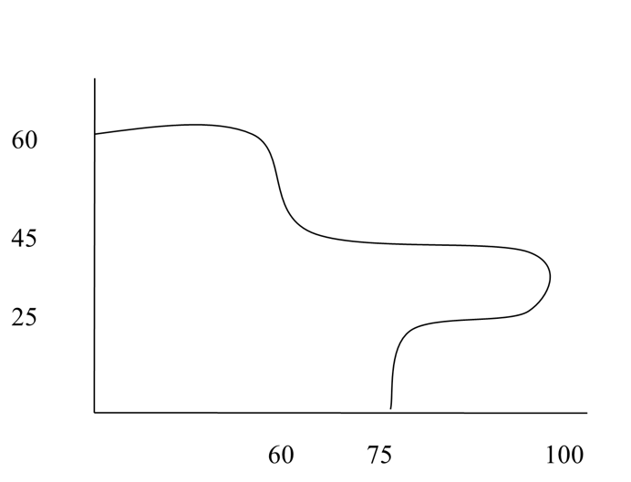
(5). The shaded area shows a plot of land available for sale. Your best estimate of the area of the land is most nearly
(A) \(2500 \ \text{m}^2\)
(B) \(4775 \ \text{m}^2\)
(C) \(5250 \ \text{m}^2\)
(D) \(6000 \ \text{m}^2\)
(6). The following data of the velocity of a body is given as a function of time.
| \(\text{Time},\ t\ (\text{s})\) | \(0\) | \(15\) | \(18\) | \(22\) | \(24\) |
|---|---|---|---|---|---|
| \(\text{Velocity}, v\ (\text{m/s})\) | \(22\) | \(24\) | \(37\) | \(25\) | \(123\) |
Using the trapezoidal rule with unequal segments, the distance covered by the body from \(t = 12 \ \text{s}\) to \(t = 18 \ \text{s}\) is
(A) \(162.90\ \text{m}\)
(B) \(166.00\ \text{m}\)
(C) \(181.70\ \text{m}\)
(D) \(436.50\ \text{m}\)
For complete solution, go to
http://nm.mathforcollege.com/mcquizzes/07int/quiz_07int_trapcontinous_solution.pdf
Problem Set
(1). Find the value of \(\displaystyle \int_{0.2}^{2.2} xe^{x} \ dx\) by using composite trapezoidal rule with two segments.
- Answer
-
\(14.033\)
(2). Find the value of \(\displaystyle \int_{- 3.4}^{2.2} x^{2}e^{x} \ dx\) by using composite trapezoidal rule with four segments.
- Answer
-
\(33.875\)
(3). The upward velocity of a rocket is given by
\[v(t) = 200\ln(t + 1) - 10t, \;\;\; t > 0 \nonumber\]
where \(t\) is given in \(\text{s}\) and \(v\) is given in \(\text{m} / \text{s}\).
a) Use composite trapezoidal rule with two segments to calculate the distance covered by the rocket from \(t = 0\ \text{s}\) to \(t = 5\ \text{s}\).
b) What is the true value of the distance covered by the rocket from \(t = 0\ \text{s}\) to \(t = 5\ \text{s}\)?
c) What is the true error in part (a)?
d) What is the relative true error in part (a)?
e) What is the absolute relative true error in percentage for part (a)?
f) Use composite trapezoidal rule with four segments to calculate the distance covered by the rocket from \(t = 0\ \text{s}\) to \(t = 5\ \text{s}\).
g) What is the absolute relative approximate error in percentage for part (e), assuming the previous approximation is from part (a)?
h) Based on the answer from part (g), how many significant digits are correct in the answer in part (g).
- Answer
-
\(a)\ 949.32\ \text{m}\)
\(b)\ 1025.1\ \text{m}\)
\(c)\ 75.790\ \text{m}\)
\(d)\ 0.073933\)
\(e)\ 7.3933\%\)
\(f)\ 1004.4\ \text{m}\)
\(g)\ 5.4865 \%\)
\(h)\ 0\)
(4). Find the value of the integral \(\displaystyle \int_{1}^{5} 3e^{-2t} \ dt\) using composite trapezoidal rule with two segments.
- Answer
-
\(0.42101\)
(5). For the integral \(\displaystyle \int_{1}^{4} xe^{-2x} \ dx\), find the following
a) Exact integral using your calculus knowledge (Hint: \(\displaystyle \int u \ dv = uv - \displaystyle \int v \ du + C\))
b) Value of integral using composite trapezoidal rule with two segments.
c) Value of integral using composite trapezoidal rule with four segments.
d) Calculate the true error for part (b) and part (c). Is the true error for part (c) approximately a quarter of the true error for part (b)? Explain.
- Answer
-
\(a)\ 0.10075\)
\(b)\ 0.12778\)
\(c)\ 0.10719\)
\(d)\ -0.027028,\ -0.00644\)
(6). In composite trapezoidal rule, if \(E_{n}\) is the true error using \(n\) (\(n \geq 1\)) segments, then the true error using composite trapezoidal rule with \(2n\) sgements approximately is ________ of \(E_{n}\).
- Answer
-
\(1/4\)
(7). The upward velocity of a body is given by
\[v(t) = \ln\left( \frac{160}{160 - 9t} \right), \;\;\; t > 0 \nonumber\]
where \(t\) is given in seconds, and \(v\) in \(\text{m}/\text{s}\).
What is the distance covered by the body from \(t = 5\) to \(t = 9\) seconds? Use composite trapezoidal rule with four segments.
- Answer
-
\(2.0280\ \text{m}\)
(8). The true error for the single application trapezoidal rule used to calculate the approximate value of the integral \(\displaystyle \int_{a}^{b} f(x) \ dx\) is given by
\[E_{t} = - \frac{(b - a)^{3}}{12}f^{\prime}(\zeta), \;\;\; a \leq \zeta \leq b \nonumber\]
For the integral\(\displaystyle \int_{3}^{6} 3e^{1.1x} \ dx\), what is the value of \(\zeta\)?
- Answer
-
\(4.7386\)
(9). The approximate value of the integral of \(\displaystyle \int_{1}^{5} f(x) \ dx\) is found by using single application trapezoidal rule as \(0.35958\). Given \(f(2) = 0.7447\), \(f(3) = 0.10454\) and \(f(4) = - 0.50730\), what is the approximate value of the integral of \(\displaystyle \int_{1}^{5} \ f(x)dx\) using the composite trapezoidal rule with two segments.
- Answer
-
\(0.38887\)
(10). The true error for trapezoidal rule used to calculate the approximate value of the integral \(\displaystyle \int_{a}^{b} f(x) \ dx\) is given by
\[E_{t} = - \frac{(b - a)^{3}}{12} f^{\prime\prime}(\zeta), \;\;\; a \leq \zeta \leq b \nonumber\]
For the integral \(\displaystyle \int_{2}^{5} (3x^{2} + dx + e) \ dx\), where constants \(d\) and \(e\) are not given to you, the single application trapezoidal rule gives the value of the integral as \(201.0\). Find the exact value of the integral.
\[E_{t} = - \frac{(b - a)^{3}}{12}f^{\prime}(\zeta), \;\;\; a \leq \zeta \leq b \nonumber\]
- Answer
-
\(187.5\)
(11). A quadrature rule is developed by a scientist:
\[\displaystyle \int_{a}^{b} f(x) \ dx \approx c_{1}f(a). \nonumber\]
The value of \(c_{1}\) is found by assuming that the formula is exact for integrals of \(f(x) = a_{0}x^{2}\), where \(a_{0}\) is an arbitrary constant. What is the value of \(c_{1}\) in terms of \(a\) and \(b\)?
- Answer
-
\(\dfrac{b^{3} - a^{3}}{3a^{2}}\)

