7.01: Prerequisites to Numerical Integration

Lesson 1: Prerequisites to Numerical Integration

Learning Objectives

After successful completion of this lesson, you should be able to:

1) define an integral,

2) use Riemann’s sum to approximately calculate integrals,

3) use Riemann’s sum and its limit to find the exact expression of integrals, and

4) find exact integrals of a few functions.

What is integration?

The dictionary definition of integration is combining parts so that they work together or form a whole. Mathematically, integration stands for finding the area under a curve from one point to another. It is represented by

\[\int_{a}^{b} f(x) \ dx\;\;\;\;\;\;\;\;\;\;\;\; (\PageIndex{1.1}) \nonumber\]

where the symbol \(\int\) is the integral sign, and \(a\) and \(b\) are the lower and upper limits of integration, respectively, the function \(f(x)\) is the integrand of the integral, and \(x\) is the variable of integration. Figure \(\PageIndex{1.1}\) represents a graphical demonstration of the concept.

Figure \(\PageIndex{1.1}\). The definite integral as the area of a region under the curve, \(\text{Area} = \int_{a}^{b} f(x) \ dx\).

Riemann Sum

Let \(f\) be defined on the closed interval \(\lbrack a,b\rbrack\), and let \(\Delta\) be an arbitrary partition of \(\lbrack a,b\rbrack\) such as: \(a = x_{0} < x_{1} < x_{2} < \ldots < x_{n - 1} < x_{n} = b\), where \(\Delta x_{i}\) is the length of the \(i^{th}\) subinterval (Figure \(\PageIndex{1.2}\)).

If \(c_{i}\) is any point in the \(i^{th}\) subinterval, then the sum

\[\sum_{i = 1}^{n}{f(c_{i})}\Delta x_{i},\ x_{i - 1} \leq c_{i} \leq x_{i}\;\;\;\;\;\;\;\;\;\;\;\; (\PageIndex{1.2}) \nonumber\]

Figure \(\PageIndex{1.2}\). Division of interval into \(n\) segments.

is called a Riemann sum of the function \(f\) for the partition \(\Delta\) on the interval \(\lbrack a,b\rbrack\). For a given partition \(\Delta\), the length of the longest subinterval is called the norm of the partition. It is denoted by \(\left\| \Delta \right\|\) (the norm of \(\Delta\)). The following limit is used to define the definite integral.

\[\lim_{\| \Delta \|\to 0} \sum_{i=1}^n f(c_i)\Delta{x_i} = I\;\;\;\;\;\;\;\;\;\;\;\; (\PageIndex{1.3}) \nonumber\]

This limit exists if and only if for any positive number \(\varepsilon\), there exists a positive number \(\delta\) such that for every partition \(\Delta\) of \(\lbrack a,b\rbrack\) with \(\left\| \Delta \right\| < \delta\), it follows that

\[\lvert I-\sum_{i=1}^nf(c_i)\Delta{x_i} \rvert < \varepsilon\;\;\;\;\;\;\;\;\;\;\;\; (\PageIndex{1.4}) \nonumber\]

for any choice of \(c_{i}\) in the \(i^{th}\) subinterval of \(\Delta\).

If the limit of a Riemann sum of \(f\) exists, then the function \(f\) is said to be integrable over \(\lbrack a,b\rbrack\) and the Riemann sum of \(f\) on \(\lbrack a,b\rbrack\) approaches the number \(I\).

\[\lim_{\left\| \Delta \right\| \rightarrow 0}\sum_{i = 1}^{n}{f\left( c_{i} \right)\Delta x_{i}} = I\;\;\;\;\;\;\;\;\;\;\;\; (\PageIndex{1.5}) \nonumber\]

where

\[I =\int_{a}^{b}{f(x) \ dx}\;\;\;\;\;\;\;\;\;\;\;\; (\PageIndex{1.6}) \nonumber\]

Audiovisual Lecture

Title: Accumulation Function

Summary: This video discusses how the accumulation function works to create a basis for numerical integration.

Example \(\PageIndex{1.1}\)

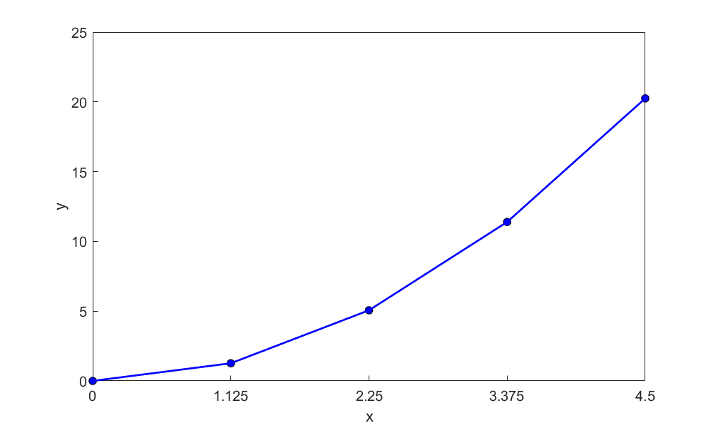
Find the area of the region between the parabola \(y = x^{2}\) and the \(x\)-axis on the interval \(\lbrack 0,4.5\rbrack\). Use the right Riemann sum with four partitions of equal segment width. Compare the value with the exact value.

Solution

We evaluate the integral for the area as a limit of Riemann sums. We sketch the region (Figure \(\PageIndex{1.3}\)), and partition \(\lbrack 0,4.5\rbrack\) into four subintervals of length

\[\begin{split} \Delta x &= \frac{4.5 - 0}{4}\\ &= 1.125 \end{split}.\]

Figure \(\PageIndex{1.3}\). Straight-line approximation of the function \(y = x^{2}\) on \(\lbrack 0,4.5\rbrack\), using 4 intervals.

The points of partition are

\[x_{0} = 0,\ x_{1} = 1.125,\ x_{2} = 2.25,\ x_{3} = 3.375,\ x_{4} = 4.5 \nonumber\]

Let us choose \(c_{i}\) to be right-hand endpoint of its subinterval. Thus,

\[c_{1} = x_{1} = 1.125,\ c_{2} = x_{2} = 2.25,\ c_{3} = x_{3} = 3.375,\ c_{4} = x_{4} = 4.5 \nonumber\]

The rectangles defined by these choices have the following areas:

\[\begin{split} f\left( c_{1} \right)\Delta x &= f\left( 1.125 \right) \times \left( 1.125 \right)\\ &= (1.125)^{2}(1.125)\\ &= 1.4238 \end{split}\]

\[\begin{split} f\left( c_{2} \right)\Delta x &= f\left( 2.25 \right) \times \left( 1.125 \right)\\ &= (2.25)^{2}(1.125)\\ &= 5.6953 \end{split}\]

\[\begin{split} f\left( c_{3} \right)\Delta x &= f\left( 3.375 \right) \times \left( 1.125 \right)\\ &= (3.375)^{2}(1.125)\\ &= 12.814 \end{split}\]

\[\begin{split} f\left( c_{4} \right)\Delta x &= f\left( 4.5 \right) \times \left( 1.125 \right)\\ &= (4.5)^{2}(1.125)\\ &= 22.781 \end{split}\]

The sum of the areas then is the approximate value of the integral

\[\begin{split} \int_{0}^{4.5}x^{2} \ dx &\approx \sum_{i = 1}^{4}{f(c_{i})\Delta x,}\\ &= {1.4238} + {5.6953} + {12.814} + {22.781}\\ &= 42.715 \end{split}\]

How does this compare with the exact value of the integral \(\displaystyle \int_{0}^{4.5}x^{2} \ dx\)?

\[\displaystyle \begin{split} \int_{0}^{4.5}x^{2} \ dx &= \left\lbrack \frac{x^{3}}{3} \right\rbrack_{0}^{4.5}\\ &= \frac{4.5^{3}}{3} - \frac{0^{3}}{3}\\ &= 30.375 \end{split}\]

Example \(\PageIndex{1.2}\)

Find the exact area of the region between the parabola \(y = x^{2}\) and the \(x\)-axis on the interval \(\lbrack 0,b\rbrack\). Use the right Riemann’s sum with equal segment widths.

Solution

Note that in Example \(\PageIndex{1.1}\) for \(y = x^{2}\) that

\[\begin{split} f\left( c_{i} \right)\Delta x &=\left(i\Delta x\right)^2\left(\Delta x \right)\\ &= i^{2}\left( {\Delta x} \right)^{3} \end{split}\;\;\;\;\;\;\;\;\;\;\;\; (\PageIndex{1.E2.1}) \nonumber\]

Thus, the sum of these areas, if the interval is divided into \(n\) equal segments, is

\[\displaystyle \begin{split} S_{n} &= \sum_{i = 1}^{n}{f(c_{i})\Delta x}\\ &= \sum_{i = 1}^{n}{i^{2}(\Delta x)^{3}}\\ &= (\Delta x)^{3}\sum_{i = 1}^{n}i^{2}\;\;\;\;\;\;\;\;\;\;\;\; (\PageIndex{1.E2.2}) \end{split}\]

Since

\[\displaystyle \Delta x = \frac{b}{n},\ \text{and}\;\;\;\;\;\;\;\;\;\;\;\; (\PageIndex{1.E2.3}) \nonumber\]

\[\displaystyle \sum_{i = 1}^{n}i^{2} = \frac{n(n + 1)(2n + 1)}{6}\;\;\;\;\;\;\;\;\;\;\;\; (\PageIndex{1.E2.4}) \nonumber\]

Substituting Equations \((\PageIndex{1.E2.3})\) and \((\PageIndex{1.E2.4})\) in Equation \((\PageIndex{1.E2.1})\), we get

\[\begin{split} S_{n} &= \frac{b^{3}}{n^{3}}\frac{n(n + 1)(2n + 1)}{6}\\ &= \frac{b^{3}}{6}\frac{2n^{2} + n + 2n + 1}{n^{2}}\\ &= \frac{b^{3}}{6}\left( 2 + \frac{3}{n} + \frac{1}{n^{2}} \right) \end{split}\]

The definition of a definite integral can now be used.

\[\displaystyle \int_{a}^{b}{f(x) \ dx}= \lim_{| \Delta{x} |\to 0} \sum_{i=1}^n f(c_i)\Delta{x} \nonumber\]

To find the area under the parabola from \(x = 0\) to \(x = b\), we have

\[\displaystyle \begin{split} \int_{0}^{b}x^{2} \ dx &= \lim_{|\Delta| \rightarrow 0}\sum_{i = 1}^{n}{f(c_{i})}{\Delta x}\\ &= \lim_{n \rightarrow \infty}S_{n}\\ &= \lim_{n \rightarrow \infty}\frac{b^{3}}{6}\left( 2 + \frac{3}{n} + \frac{1}{n^{2}} \right)\\ &= \frac{b^{3}}{6}\left( 2 + 0 + 0 \right)\\ &= \frac{b^{3}}{3} \end{split}\]

Mean Value of a Function

The mean value \(\overline{f}\) of a function \(f\) in an interval \(\lbrack a,b\rbrack\) is given by

\[\displaystyle \overline{f} = \frac{1}{b - a}\int_{a}^{b}{f(x) \ dx}\;\;\;\;\;\;\;\;\;\;\;\; (\PageIndex{1.7}) \nonumber\]

Example \(\PageIndex{1.3}\)

Find the average value of \(f(x) = (x - 1)^{2}\) over the interval \(\lbrack 0,3\rbrack\). At what point in the given interval does the function assume this average value?

Solution

\[\begin{split} \overline{f} &= \frac{1}{b - a}\int_{a}^{b}{f\left( x \right) \ dx}\\ &= \frac{1}{3 - 0}\int_{a}^{b}{\left( x - 1 \right)^{2} \ dx}\\ &= \frac{1}{3 - 0}\left\lbrack \frac{(x - 1)^{3}}{3} \right\rbrack_{0}^{3}\\ &= \frac{1}{3 - 0}\left\lbrack \frac{\left( 3 - 1 \right)^{3}}{3} - \frac{\left( 0 - 1 \right)^{3}}{3} \right\rbrack\\ &= 1 \end{split}\]

The average value of the function \(f\) over the interval \(\lbrack 0,3\rbrack\) is \(1\).

Figure \(\PageIndex{1.4}\). The function \(f(x) = (x - 1)^{2}\).

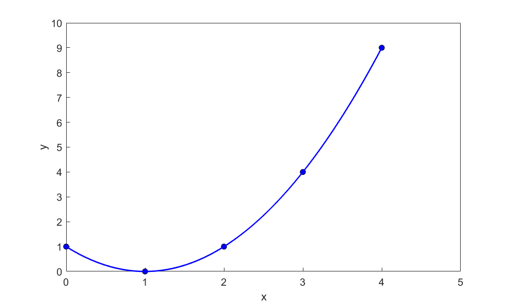
The function assumes the average value at the points where

\[(x-1)^2=1 \nonumber\]

\[x^2-2x+1=1 \nonumber\]

\[x^2-2x=0 \nonumber\]

\[x(x-2)=0 \nonumber\]

\[x=0\ \text{and}\ x=2 \nonumber\]

As evident from Figure \(\PageIndex{1.4}\), the function value is \(1\) at \(x=0\) and \(x=2\).

Table \(\PageIndex{1.1}\) lists a number of standard indefinite integral forms.

Table \(\PageIndex{1.1}\). A brief table of integrals.

Integrals
\(\displaystyle \int dx=x+C\)
\(\displaystyle \int af(x) \ dx=a\int f(x) \ dx+C\)
\(\displaystyle \int [u(x)\pm v(x) \ dx]=\int u(x)dx \pm \int v(x) \ dx+C\)
\(\displaystyle \int x^n \ dx = \frac{x^n+1}{n+1}+C\)
\(\displaystyle \int u \ dv=uv-\int v \ du+C\)
\(\displaystyle \int \frac{dx}{ax+b}=\frac{1}{a}\ln|ax+b| +C\)
\(\displaystyle \int a^x \ dx=\frac{a^x}{\ln a}+C\)
\(\displaystyle \int e^{ax} \ dx=\frac{e^{ax}}{a}+C\)
\(\displaystyle \int \cos{x} \ dx=\sin{x}+C\)
\(\displaystyle \int \sin{x} \ dx=-\cos{x}+C\)
\(\displaystyle \int \tan{x} \ dx=-ln{|\cos{x}|}+C=ln{|\sec{x}|}+C\)
\(\displaystyle\int \sec(ax) \ dx =\frac{1}{a} \ln|\sec(ax)+ tan(ax)|+C\)
\(\displaystyle \int \cot{x} \ dx=-ln{|\csc{x}|}+C=ln{|\sin{x}|}+C\)
\(\displaystyle \int{\sec}^2{a}x \ dx=\frac{1}{a}\tan(ax)+C\)
\(\displaystyle \int \sec(x) \tan(x) \ dx=\sec(x)+C\)
\(\displaystyle \int \csc(x)\cot(x) \ dx=-\csc(x)+C\)

Multiple Choice Test

(1). Physically, integrating \(\displaystyle \int_{a}^{b}{f(x) \ dx}\) means finding the

(A) area under the curve from \(a\) to \(b\)

(D) area to the left of point \(a\)

(C) area to the right of point \(b\)

(D) area above the curve from \(a\) to \(b\)

(2). The mean value of a function \(f(x)\) from \(a\) to \(b\) is given by

(A) \(\displaystyle \frac{f(a) + f(b)}{2}\)

(D) \(\displaystyle \frac{f(a) + 2f\left(\displaystyle \frac{a + b}{2} \right) + f(b)}{4}\)

(C) \(\displaystyle \int_{a}^{b}{f(x) \ dx}\)

(D) \(\displaystyle \frac{\displaystyle \int_{a}^{b} f(x) \ dx}{b - a}\)

(3). The exact value of \(\displaystyle \int_{0.2}^{2.2} xe^{x} \ dx\) is most nearly

(A) \(7.8036\)

(D) \(11.807\)

(C) \(14.034\)

(D) \(19.611\)

(4). \(\displaystyle \int_{0.2}^{2} f(x) \ dx\) for

\[f(x) = \begin{cases} x, \;\;\;\;\;\;\;\;\;\;\; 0 \leq x \leq 1.2 \\ x^{2}, \;\;\;\;\;\;\;\;\;\; 1.2 < x \leq 2.4 \end{cases} \nonumber\]

is most nearly

(A) \(1.9800\)

(D) \(2.6640\)

(C) \(2.7907\)

(D) \(4.7520\)

(5). The area of a circle of radius \(a\) can be found by which of the following integrals?

(A) \(\displaystyle \int_{0}^{a} \left( a^{2} - x^{2} \right) \ dx\)

(D) \(\displaystyle \int_{0}^{2\pi} \sqrt{a^{2} - x^{2}} \ dx\)

(C) \(\displaystyle 4\int_{0}^{a} \sqrt{a^{2} - x^{2}} \ dx\)

(D) \(\displaystyle \int_{0}^{a} \sqrt{a^{2} - x^{2}} \ dx\)

(6). Velocity distribution of a fluid flow through a pipe varies along the radius and is given by \(v(r)\). The flow rate through the pipe of radius \(a\) is given by

(A) \(\displaystyle \pi v(a)a^{2}\)

(D) \(\displaystyle \pi\frac{v(0) + v(a)}{2}a^{2}\)

(C) \(\displaystyle \int_{0}^{a} v(r) \ dr\)

(D) \(\displaystyle 2\pi\int_{0}^{a} v(r)r \ dr\)

For complete solution, go to

http://nm.mathforcollege.com/mcquizzes/07int/quiz_07int_background_solution.pdf