3.2: Using Derivatives to Describe Families of Functions

Learning Objectives

In this section, we strive to understand the ideas generated by the following important questions:

• Given a family of functions that depends on one or more parameters, how does the shape of the graph of a typical function in the family depend on the value of the parameters?
• How can we construct first and second derivative sign charts of functions that depend on one or more parameters while allowing those parameters to remain arbitrary constants?

Mathematicians are often interested in making general observations, say by describing patterns that hold in a large number of cases. For example, think about the Pythagorean Theorem: it doesn’t tell us something about a single right triangle, but rather a fact about every right triangle, thus providing key information about every member of the right triangle family. In the next part of our studies, we would like to use calculus to help us make general observations about families of functions that depend on one or more parameters. People who use applied mathematics, such as engineers and economists, often encounter the same types of functions in various settings where only small changes to certain constants occur. These constants are called parameters. We are already familiar with certain families of functions. For example,

\[f (t) = a \sin(b(t − c)) + d\]

is a stretched and shifted version of the sine function with amplitude \(a\), period \(2π b\), phase shift \(c\), and vertical shift \(d\). We understand from experience with trigonometric functions that a affects the size of the oscillation, b the rapidity of oscillation, and c where the oscillation starts, as shown in Figure 3.13, while d affects the vertical positioning of the graph. In addition, there are several basic situations that we already understand completely. For instance, every function of the form y = mx + b is a line with slope m and y-intercept (0, b). Note that the form y = mx + b allows us to consider every possible line by using two parameters (except for vertical lines which are of the form x = a). Further, we understand that the value of m affects the line’s steepness and whether the line rises or falls from left to right, while the value of b situates the line vertically on the coordinate axes. For other less familiar families of functions, we would like to use calculus to understand and classify where key behavior occurs: where members of the family are increasing or decreasing, concave up or concave down, where relative extremes occur, and more, all

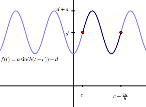
Figure 3.13: The graph of f (t) = a sin(b(t − c)) + d based on parameters a, b, c, and d.

in terms of the parameters involved. To get started, we revisit a common collection of functions to see how calculus confirms things we already know.

Preview Activity \(\PageIndex{1}\)

Let a, h, and k be arbitrary real numbers with a , 0, and let f be the function given by the rule f (x) = a(x − h) 2 + k.

1. What familiar type of function is f? What information do you know about f just by looking at its form? (Think about the roles of a, h, and k.)
2. Next we use some calculus to develop familiar ideas from a different perspective. To start, treat a, h, and k as constants and compute f 0 (x).
3. Find all critical numbers of f . (These will depend on at least one of a, h, and k.)
4. Assume that a < 0. Construct a first derivative sign chart for f .
5. Based on the information you’ve found above, classify the critical values of f as maxima or minima. ./

Describing families of functions in terms of parameters Given a family of functions that depends on one or more parameters, our goal is to describe the key characteristics of the overall behavior of each member of the familiy in terms of those parameters. By finding the first and second derivatives and constructing first and second derivative sign charts (each of which may depend on one or more of the 176 parameters), we can often make broad conclusions about how each member of the family will appear. The fundamental steps for this analysis are essentially identical to the work we did in Section 3.1, as we demonstrate through the following example.

Example \(\PageIndex{1}\)

Consider the two-parameter family of functions given by g(x) = axe−bx , where a and b are positive real numbers. Fully describe the behavior of a typical member of the family in terms of a and b, including the location of all critical numbers, where g is increasing, decreasing, concave up, and concave down, and the long term behavior of g.

Solution.

We begin by computing g 0 (x). By the product rule, g 0 (x) = ax d dx f e −bx g + e −bx d dx [ax], and thus by applying the chain rule and constant multiple rule, we find that g 0 (x) = axe−bx(−b) + e −bx(a). To find the critical numbers of g, we solve the equation g 0 (x) = 0. Here, it is especially helpful to factor g 0 (x). We thus observe that setting the derivative equal to zero implies 0 = ae−bx(−bx + 1). Since we are given that a , 0 and we know that e −bx , 0 for all values of x, the only way the preceding equation can hold is when −bx + 1 = 0. Solving for x, we find that x = 1 b , and this is therefore the only critical number of g. Now, recall that we have shown g 0 (x) = ae−bx(1−bx) and that the only critical number of g is x = 1 b . This enables us to construct the first derivative sign chart for g that is shown in Figure 3.14.

Figure 3.14: The first derivative sign chart for g(x) = axe−bx .

Note particularly that in g 0 (x) = ae−bx(1 − bx), the term ae−bx is always positive, so the sign depends on the linear term (1 − bx), which is zero when x = 1 b . Note that this line has negative slope (−b), so (1 − bx) is positive for x < 1 b and negative for x > 1 b . Hence we can not only conclude that g is always increasing for x < 1 b and decreasing for x > 1 b , but also that g has a global maximum at ( 1 b , g( 1 b )) and no local minimum. We turn next to analyzing the concavity of g. With g 0 (x) = −abxe−bx + ae−bx, we differentiate to find that g 00(x) = −abxe−bx(−b) + e −bx(−ab) + ae−bx(−b). Combining like terms and factoring, we now have g 00(x) = ab2 xe−bx − 2abe−bx = abe−bx(bx − 2). Similar to our work with the first derivative, we observe that abe−bx is always positive,

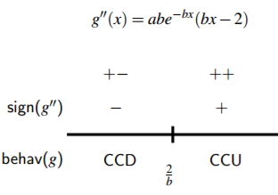
Figure 3.15: The second derivative sign chart for g(x) = axe−bx .

and thus the sign of g 00 depends on the sign of (bx − 2), which is zero when x = 2 b . Since (bx − 2) represents a line with positive slope (b), the value of (bx − 2) is negative for x < 2 b and positive for x > 2 b , and thus the sign chart for g 00 is given by the one shown in Figure 3.15. Thus, g is concave down for all x < 2 b and concave up for all x > 2 b . Finally, we analyze the long term behavior of g by considering two limits. First, we note that limx→∞ g(x) = limx→∞ axe−bx = limx→∞ ax e bx . Since this limit has indeterminate form ∞ ∞ , we can apply L’Hopital’s Rule and thus find that limx→∞ g(x) = 0. In the other direction, limx→−∞ g(x) = limx→−∞ axe−bx = −∞, since ax → −∞ and e −bx → ∞ as x → −∞. Hence, as we move left on its graph, g decreases without bound, while as we move to the right, g(x) → 0. 178 All of the above information now allows us to produce the graph of a typical member of this family of functions without using a graphing utility (and without choosing particular values for a and b), as shown in Figure 3.16.

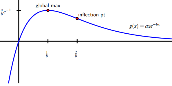
Figure 3.16: The graph of g(x) = axe−bx .

We note that the value of b controls the horizontal location of the global maximum and the inflection point, as neither depends on a. The value of a affects the vertical stretch of the graph. For example, the global maximum occurs at the point ( 1 b , g( 1 b )) = ( 1 b , a b e −1 ), so the larger the value of a, the greater the value of the global maximum.

The kind of work we’ve completed in Example 3.3 can often be replicated for other families of functions that depend on parameters. Normally we are most interested in determining all critical numbers, a first derivative sign chart, a second derivative sign chart, and some analysis of the limit of the function as x → ∞. Throughout, we strive to work with the parameters as arbitrary constants. If stuck, it is always possible to experiment with some particular values of the parameters present to reduce the algebraic complexity of our work. The following sequence of activities offers several key examples where we see that the values of different parameters substantially affect the behavior of individual functions within a given family.

Activity \(\PageIndex{2}\)

Consider the family of functions defined by p(x) = x 3 − ax, where a , 0 is an arbitrary constant.

1. Find p 0 (x) and determine the critical numbers of p. How many critical numbers does p have?
2. Construct a first derivative sign chart for p. What can you say about the overall 179 behavior of p if the constant a is positive? Why? What if the constant a is negative? In each case, describe the relative extremes of p.
3. Find p 00(x) and construct a second derivative sign chart for p. What does this tell you about the concavity of p? What role does a play in determining the concavity of p?
4. Without using a graphing utility, sketch and label typical graphs of p(x) for the cases where a > 0 and a < 0. Label all inflection points and local extrema.
5. Finally, use a graphing utility to test your observations above by entering and plotting the function p(x) = x 3 − ax for at least four different values of a. Write several sentences to describe your overall conclusions about how the behavior of p depends on a. C

Activity \(\PageIndex{3}\)

Consider the two-parameter family of functions of the form h(x) = a(1 − e −bx), where a and b are positive real numbers.

1. Find the first derivative and the critical numbers of h. Use these to construct a first derivative sign chart and determine for which values of x the function h is increasing and decreasing.
2. Find the second derivative and build a second derivative sign chart. For which values of x is a function in this family concave up? concave down?
3. What is the value of limx→∞ a(1 − e −bx)? limx→−∞ a(1 − e −bx)?
4. How does changing the value of b affect the shape of the curve?
5. Without using a graphing utility, sketch the graph of a typical member of this family. Write several sentences to describe the overall behavior of a typical function h and how this behavior depends on a and b. C

Activity \(\PageIndex{4}\)

Let L(t) = A 1 + ce−kt , where A, c, and k are all positive real numbers.

1. Observe that we can equivalently write L(t) = A(1 + ce−kt) −1 . Find L 0 (t) and explain why L has no critical numbers. Is L always increasing or always decreasing? Why?
2. Given the fact that L 00(t) = Ack2 e −kt ce−kt − 1 (1 + ce−kt) 3 , 180 find all values of t such that L 00(t) = 0 and hence construct a second derivative sign chart. For which values of t is a function in this family concave up? concave down?
3. What is the value of limt→∞ A 1 + ce−kt ? limt→−∞ A 1 + ce−kt ?
4. Find the value of L(x) at the inflection point found in (b).
5. Without using a graphing utility, sketch the graph of a typical member of this family. Write several sentences to describe the overall behavior of a typical function L and how this behavior depends on A, c, and kcritical number. (f) Explain why it is reasonable to think that the function L(t) models the growth of a population over time in a setting where the largest possible population the surrounding environment can support is A.

Summary

In this section, we encountered the following important ideas:

• Given a family of functions that depends on one or more parameters, by investigating how critical numbers and locations where the second derivative is zero depend on the values of these parameters, we can often accurately describe the shape of the function in terms of the parameters.
• In particular, just as we can created first and second derivative sign charts for a single function, we often can do so for entire families of functions where critical numbers and possible inflection points depend on arbitrary constants. These sign charts then reveal where members of the family are increasing or decreasing, concave up or concave down, and help us to identify relative extremes and inflection points. critical number

Contributors and Attributions

• Matt Boelkins (Grand Valley State University), David Austin (Grand Valley State University), Steve Schlicker (Grand Valley State University)