
7.5: Modeling with Differential Equations


- Last updated
- Apr 4, 2022
- Save as PDF
( \newcommand{\kernel}{\mathrm{null}\,}\)
Learning Objectives
In this section, we strive to understand the ideas generated by the following important questions:
- How can we use differential equations to describe phenomena in the world around us?
- How can we use differential equations to better understand these phenomena?
In our work to date, we have seen several ways that differential equations arise in the natural world, from the growth of a population to the temperature of a cup of coffee. In this section, we will look more closely at how differential equations give us a natural way to describe various phenomena. As we’ll see, the key is to focus on understanding the different factors that cause a quantity to change.
Preview Activity 7.5.1
Any time that the rate of change of a quantity is related to the amount of a quantity, a differential equation naturally arises. In the following two problems, we see two such scenarios; for each, we want to develop a differential equation whose solution is the quantity of interest.
- Suppose you have a bank account in which money grows at an annual rate of 3%.
- If you have $10,000 in the account, at what rate is your money growing?
- Suppose that you are also withdrawing money from the account at $1,000 per year. What is the rate of change in the amount of money in the account? What are the units on this rate of change?
- Suppose that a water tank holds 100 gallons and that a salty solution, which contains 20 grams of salt in every gallon, enters the tank at 2 gallons per minute.
- How much salt enters the tank each minute?
- Suppose that initially there are 300 grams of salt in the tank. How much salt is in each gallon at this point in time?
- Finally, suppose that evenly mixed solution is pumped out of the tank at the rate of 2 gallons per minute. How much salt leaves the tank each minute?
- What is the total rate of change in the amount of salt in the tank?
Developing a Differential Equation
Preview activity 7.5.1 demonstrates the kind of thinking we will be doing in this section. In each of the two examples we considered, there is a quantity, such as the amount of money in the bank account or the amount of salt in the tank, that is changing due to several factors. The governing differential equation results from the total rate of change being the difference between the rate of increase and the rate of decrease.
Example 7.5.1: Lake Michigan
In the Great Lakes region, rivers flowing into the lakes carry a great deal of pollution in the form of small pieces of plastic averaging 1 millimeter in diameter. In order to understand how the amount of plastic in Lake Michigan is changing, construct a model for how this type pollution has built up in the lake.
Solution
First, some basic facts about Lake Michigan.
- The volume of the lake is 5×10¹² cubic meters.
- Water flows into the lake at a rate of 5×10¹⁰ cubic meters per year. It flows out of the lake at the same rate.
- Each cubic meter flowing into the lake contains roughly 3×10⁻⁸ cubic meters of plastic pollution.
Let’s denote the amount of pollution in the lake by P(t), where P is measured in cubic meters of plastic and t in years. Our goal is to describe the rate of change of this function; in other words, we want to develop a differential equation describing P(t).
First, we will measure how P(t) increases due to pollution flowing into the lake. We know that 5×10¹⁰ cubic meters of water enters the lake every year and each cubic meter of water contains 3×10⁻⁸ cubic meters of pollution. Therefore, pollution enters the lake at the rate of
(5⋅1010m3wateryear)⋅(3⋅10−8m3plasticm3water)=1.5⋅103
Second, we will measure how P(t) decreases due to pollution flowing out of the lake. If the total amount of pollution is P cubic meters and the volume of Lake Michigan is 5⋅1012 cubic meters then the concentration of plastic pollution in Lake Michigan is
P5⋅1012 cubic meters of plastic per cubic meter of water.
Since 5⋅1010 cubic meters of water flow out each year, then the plastic pollution leaves the lake at the rate of
(P5⋅1012m3plasticm3water)⋅(5⋅1010m3wateryear)=P100 cubic meters of plastic per cubic meter of water.
The total rate of change of P is thus the difference between the rate at which pollution enters the lake minus the rate at which pollution leaves the lake; that is,
dPdt=1.5⋅103−P100=1100(1.5⋅105−P).
We have now found a differential equation that describes the rate at which the amount of pollution is changing. To better understand the behavior of P(t), we now apply some of the techniques we have recently developed.
Since this is an autonomous differential equation, we can sketch dP/dt as a function of P and then construct a slope field, as shown in Figure 7.5.1.
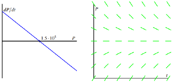
Figure 7.5.1: Plots of dPdt vs. P and the slope field for the differential equation dPdt=1100(1.5⋅105−P).
These plots both show that P=1.5⋅105 is a stable equilibrium. Therefore, we should expect that the amount of pollution in Lake Michigan will stabilize near 1.5⋅105 cubic meters of pollution. Next, assuming that there is initially no pollution in the lake, we will solve the initial 6 and we assume that each cubic meter of water that flows out carries with it the plastic pollution it contains value problem
dPdt=1100(1.5⋅105−P), P(0)=0.
Separating variables, we find that
11.5⋅105−PdPdt=1100.
Integrating with respect to t, we have
∫11.5⋅105−PdPdtdt=∫1100 dt
and thus changing variables on the left and antidifferentiating on both sides, we find that
∫dP1.5⋅105P=∫1100dt
−ln|1.5⋅105−P|=1100t+C
Finally, multiplying both sides by −1 and using the definition of the logarithm, we find that
1.5⋅105−P=Ce−t/100.
This is a good time to determine the constant C. Since P=0 when t=0, we have
1.5⋅105−0=Ce0=C.
In other words, C=1.5×10⁵
Using this value of C in Equation (7.1) and solving for P, we arrive at the solution
P(t)=1.5⋅105(1−e−t/100)
Superimposing the graph of P on the slope field we saw in Figure 7.5.1, we see, as shown in Figure 7.5.2 We see that, as expected, the amount of plastic pollution stabilizes around 1.5⋅105 cubic meters.
There are many important lessons to learn from Example 7.5.1. Foremost is how we can develop a differential equation by thinking about the “total rate = rate in - rate out” model. In addition, we note how we can bring together all of our available understanding (plotting dPdt vs. P, creating a slope field, solving the differential equation) to see how the differential equation describes the behavior of a changing quantity.
Of course, we can also explore what happens when certain aspects of the problem change. For instance, let’s suppose we are at a time when the plastic pollution entering
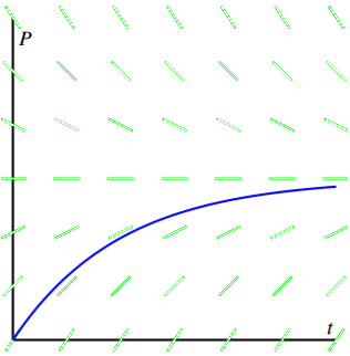
Figure 7.5.2: The solution P(t) and the slope field for the differential equation dPdt=1100(1.5×10⁵−P).
Lake Michigan has stabilized at 1.5×10⁵ cubic meters, and that new legislation is passed to prevent this type of pollution entering the lake. So, there is no longer any inflow of plastic pollution to the lake. How does the amount of plastic pollution in Lake Michigan now change? For example, how long does it take for the amount of plastic pollution in the lake to halve?
Restarting the problem at time t=0, we now have the modified initial value problem
dPdt=−1100P, P(0)=1.5⋅105.
It is a straightforward and familiar exercise to find that the solution to this equation is P(t)=1.5⋅105e−t/100. The time that it takes for half of the pollution to flow out of the lake is given by T where P(T)=0.75⋅105. Thus, we must solve the equation
0.75×105=1.5×10⁵e−T/100,
or
12=e−T/100.
It follows that
T=−100ln(12)≈69.3, years.
In the upcoming activities, we explore some other natural settings in which differential equation model changing quantities.
Activity 7.5.1: Accrued Savings
Suppose you have a bank account that grows by 5% every year. Let A(t) be the amount of money in the account in year t.
- What is the rate of change of A with respect to t?
- Suppose that you are also withdrawing $10,000 per year. Write a differential equation that expresses the total rate of change of A.
- Sketch a slope field for this differential equation, find any equilibrium solutions, and identify them as either stable or unstable. Write a sentence or two that describes the significance of the stability of the equilibrium solution.
- Suppose that you initially deposit $100,000 into the account. How long does it take for you to deplete the account?
- What is the smallest amount of money you would need to have in the account to guarantee that you never deplete the money in the account?
- If your initial deposit is $300,000, how much could you withdraw every year without depleting the account?
Activity 7.5.2: Morphine
A dose of morphine is absorbed from the bloodstream of a patient at a rate proportional to the amount in the bloodstream.
- Write a differential equation for M(t), the amount of morphine in the patient’s bloodstream, using k as the constant proportionality.
- Assuming that the initial dose of morphine is M0, solve the initial value problem to find M(t). Use the fact that the half-life for the absorption of morphine is two hours to find the constant k.
- Suppose that a patient is given morphine intravenously at the rate of 3 milligrams per hour. Write a differential equation that combines the intravenous administration of morphine with the body’s natural absorption.
- Find any equilibrium solutions and determine their stability.
- Assuming that there is initially no morphine in the patient’s bloodstream, solve the initial value problem to determine M(t). What happens to M(t) after a very long time?
- To what rate should a doctor reduce the intravenous rate so that there is eventually 7 milligrams of morphine in the patient’s bloodstream?
Summary
In this section, we encountered the following important ideas:
- Differential equations arise in a situation when we understand how various factors cause a quantity to change.
- We may use the tools we have developed so far—slope fields, Euler’s methods, and our method for solving separable equations—to understand a quantity described by a differential equation.