part0000

We thank some journal publishers who allow limited use of figures from papers in their journals either without charge (Nature, Entomological Society of America, Behaviour, Journal of Animal Ecology, Antibiotics and Chemotherapy) or with a small charge (Science). We also thank several individuals who have given permission to use their material.

Wikipedia and government web sites and a few other sites have been very useful in providing some text images.

This text is a product of a two-semester calculus course for life sciences students in which students gathered biological data in a laboratory setting that was used to motivate the concepts of calculus. The book contains data from experiments, but does not require that students do laboratory experiments.

Several MATLAB programs are provided for exercises and for explicit statement of a method. All but two or three are short, almost in the form of pseudocode, and can be readily translated to other technology, including that of programmable hand calculators.

All of the graphs in the text were created using MATLAB licensed to the Department of Mathematics at Iowa State University, Ames, Iowa. The text was written in LaTeX using the WinEdt software, also licensed to the Department of Mathematics at Iowa State University, Ames, Iowa. More than 50 color figures were converted from .jpg to .eps using http: //image.online-convert.com/convert-to-eps.

About Calculus for the Life Sciences: A Modeling Approach

Our writing is based on three premises. First, life sciences students are motivated by and respond well to actual data related to real life sciences problems. Second, the ultimate goal of calculus in the life sciences primarily involves modeling living systems with difference and differential equations. Understanding the concepts of derivative and integral are crucial, but the ability to compute a large array of derivatives and integrals is of secondary importance. Third, the depth of calculus for life sciences students should be comparable to that of the traditional physics and engineering calculus course; else life sciences students will be short changed and their faculty will advise them to take the ‘best’ (engineering) course.

The common pedagogical goal of converting students from passive listeners or readers to active problem solvers is fundamental to this text. Distributed throughout are ‘Explore’ problems that expand the text and in some cases are crucial to the development of the material.

In our text, mathematical modeling and difference and differential equations lead, closely follow, and extend the elements of calculus. Chapter one introduces mathematical modeling in which students write descriptions of some observed processes and from these descriptions derive first order linear difference equations whose solutions can be compared with the observed data. In chapters in which the derivatives of algebraic, exponential, or trigonometric functions are defined, biologically motivated differential equations and their solutions are included. The chapter on partial derivatives includes a section on the diffusion partial differential equation. There is a chapter on systems of two difference equations.

The derivative and integral are carefully defined and distinguished from the discrete data of the laboratories. The analysis of calculus thus extends the discrete laboratory observations. The Fundamental Theorem of Calculus is clearly explained on a purely analytical basis; it seems to not lend itself to laboratory exercise. An ‘Explore’ problem asks students to give reasons for the steps in the analysis.

We have also included some traditional and not necessarily biological applications of the derivative and integral (max-min, related rates, area, volume, surface area problems) because they have proved over many years to be useful to students in gaining an understanding of calculus.

The authors are grateful to the Division of Undergraduate Education of the National Science Foundation for support in 1994-1996 to develop the course on which this text is based. We are also grateful to numerous students who learned from the early versions of the text and to faculty colleagues, Warren Dolphin, Brin Keller, and Gail Johnston, who collaborated in the development and teaching of the course.

All of the graphs in the text were created using MATLAB licensed to the Department of Mathematics at Iowa State University, Ames, Iowa. The text was

written in LaTeX using the WinEdt software, also licensed to the Department of Mathematics at Iowa State University, Ames, Iowa. More than 50 color figures were converted from .jpg to .eps using Online-Convert.com.

We thank some journal publishers who allow limited use of figures from papers in their journals either without charge (Nature, Entomological Society of America, Behaviour, Journal of Animal Ecology, Antibiotics and Chemotherapy) or with a small charge (Science). A number of our figures were downloaded from Wikipedia and government web sites

With amazing insight and energy, Louis Gross and John Jungck have led and supported the mathematics in biology education community for almost a quarter of a century, and they have supported our program in several ways. Lou Gross maintains several web resources, links to which may be found on his personal web page. John Jungck’s work is well represented on the Bioquest web page.

JLC is particularly grateful to Carolyn, his wife, who has strongly supported the writing of this work and to Charles DeLisi, Jay Berzofsky, and Hanah Margalit who introduced him to real and incredibly interesting biology problems. He was extraordinarily fortunate to study under Professor R. L. Moore at the University of Texas who greatly enhanced his thinking in mathematics and in other areas of interest.

About the Authors

James L. Cornette taught university level mathematics for 45 years as a graduate student at the University of Texas and a faculty member at Iowa State University. His research includes point set topology, genetics, biomolecular structure, viral dynamics, and paleontology and has been published in Fundamenta Mathematica, Transactions of the American Mathematical Society, Proceedings of the American Mathematical Society, Heredity, Journal of Mathematical Biology, Journal of Molecular Biology, and the biochemistry, the geology, and the paleontology sections of the Proceedings of the National Academy of Sciences, USA. Dr. Cornette received an Iowa State University Outstanding Teacher Award in 1973, was a Fulbright lecturer at the Universiti Kebangsaan Malaysia in 1973-74, worked in the Laboratory of Mathematical Biology in the National Cancer Institute, NIH in 1985-1987, and and was named University Professor at Iowa State University in 1998. He retired in 2000 and began graduate study at the University of Kansas where he earned a master’s degree in Geology (Paleontology) in 2002. Presently he is a volunteer in the Earth Sciences Division of the Denver Museum of Nature and Science.

Ralph A. Ackerman is a professor in the Department of Ecology, Evolution and Organismal Biology at Iowa State University. He has been a faculty member since 1981 where his research focuses on describing and understanding the environmental physiology of vertebrate embryos, especially reptile and bird embryos. His approach is typically interdisciplinary and employs both theoretical and experimental techniques to generate and test hypotheses. He currently examines water exchange by reptile eggs during incubation and temperature dependent sex determination in reptiles.

Answers to select exercises are available at the web site, http: / / cornette.public.iastate.edu/CLS.html

Basic formulas appear on the next two pages.

F'(a) [C]’ =

\ti =

.. F{b)-F{a) ,. F(a + /i)-F(a) = hm = hm

b^a 0 — a h^O

0

b — a

Primary Formulas

h

[e*]’ = e* [sin t]’ = cos t

[In t]’ = j [cos £]’ = — sin t

Combination Rules

[u(t) x v(t)]’ = u'(t) x v(t) + u(t) x c'(t)

[C x «(*)]’ [u(t)+v(t)]’

C x u ‘(t) u'(t)+u'(t)

u{t)

v(t)_

[G(u(t))F = G'(u(t)) x u'{t)

v(t) x u'(i) – u(t) x

Chain Rule Special Cases

[(u(t)y

D u(t)

pn( «(*))]’

< ‘ x //'(/) x u'{t)

1

M «(*))]’ =

[«*(«(*))]’ =

cos( -u(t)) x it'(t) — sin(u(i)) x -u'(t)

u(t)

One special case of the chain rule is very important to the biological sciences.

e kt x k

Solutions to Difference Equations

Kx t =>• x t = x 0 K l

x t+ 2+px t+1 + qx t = 0

A r\ + B r\ where T\ and r 2

x t = < or are the roots to

Ar\ + Btr{ r 2 +pr + q = 0

Solutions to Differential (or Derivative) Equations

x'(t) = kx(t) => x(t)

x”(t)+px'(t) + qx(t) = 0 =>-

x(0)e

fct

Ae rit + 5e r2t or

Ae rit + Bte rit

where ri and r 2 are the roots to r 2 +pr + q = 0

Ja ||A||—>0 Jb Ja Ja

f ( /(f) + #(f)) dt = f fit) dt + f git) dt, f cf(t) dt = c I’ f{t) dt

J a J a J a J a J a

r f^ dt + f f^ dt = j b fn) dt f +c fn c )dt= f f^ dt

J a Jc J a J a+c J a

fit) < git) for all f in [a, b] =>• f f(t) dt < f git) dt

J a J a

G{x) = f fit) dt =► G\x) = fix), f F\t) dt = Fib) – F(a) = F(t) \\ ,

J a J a

f Odu = C f e u du = e u + C f sin u du = — cos u + C

f u n du = ‘ M ^- + C n^-1 / – du — In u + C f cos udu = sin u + C

n+l

J fit) x g’it) dt = fit) x git) – J f\t) x git) dt

If u = g(z) and jf /(«) d« = jf fig(z))^(z)dz

fb / x5(a;)A(a;) dx

Moment of mass = / (x — c)5(x)^4(x) dx. Center of mass = c = .

/ S(x)A(x) dx

J a

Length of the graph of / is / \Jl + ( fix) ) 2 dx

J a

Solids of Revolution: Volume = n if\x)) 2 dx Surface = f 2tt/(x) yl + ( f (x) ) 2 dx

J a J a

roc rR r r rb rg(x)

/ /(f)df=lim / /(f) df / FiP)dA= / Fix,y)dydx

J a R-^oo J a J R J J a J f( x )

Contents

1 Mathematical Models of Biological Processes 1

1.1 Experimental data, bacterial growth 3

1.1.1 Steps towards building a mathematical model 5

1.1.2 Concerning the validity of a model 9

1.2 Solution XoP M -P t =rP t 11

1.3 Sunlight depletion in a lake or ocean 14

1.4 Doubling Time and Half-Life 22

1.5 Quadratic Solution Equations: Mold growth 25

1.6 Constructing a Mathematical Model of Penicillin Clearance 32

1.7 Movement toward equilibrium 35

1.8 Solution to the dynamic equation P M – P t = rP t + b 41

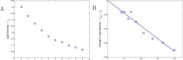
1.9 Light Decay with Distance 42

1.10 Data modeling vs mathematical models 46

1.11 Summary 49

2 Descriptions of Biological Patterns 53

2.1 Environmental Sex Determination in Turtles 53

2.2 Functions and Simple Graphs 55

2.2.1 Three definitions of “Function” 55

2.2.2 Simple graphs 58

2.2.3 Functions in other settings 62

2.3 Function notation 64

2.4 Polynomial functions 67

2.5 Least squares fit of polynomials to data 70

2.6 New functions from old 74

2.6.1 Arithmetic combinations of functions 74

2.6.2 The inverse of a function 76

2.6.3 Finding the equation of the inverse of a function 79

2.7 Composition of functions 85

Formulas for function composition 86

2.8 Periodic functions and oscillations 91

2.8.1 Trigonometric Functions 98

3 The Derivative 103

3.1 Tangent to the graph of a function 104

3.2 Limit and rate of change as a limit 123

3.3 The derivative function, F° 134

3.4 Mathematical models using the derivative 143

3.4.1 Mold growth 143

3.4.2 Difference Equations and Differential Equations 144

3.4.3 Chemical kintetics 145

Butyl chloride 146

3.5 Derivatives of Polynomials, Sum and Constant Factor Rules 149

3.5.1 Velocity as a derivative 154

3.5.2 Local Maxima and Local Minima 155

3.6 The second derivative and higher order derivatives 162

3.6.1 Falling objects 165

3.7 Left and right limits and derivatives; limits involving infinity 170

3.8 Summary of Chapter 3, The Derivative 173

4 Continuity and the Power Chain Rule 176

4.1 Continuity 176

4.2 The Derivative Requires Continuity 184

4.3 The generalized power rule 187

4.3.1 The Power Chain Rule 191

4.4 Applications of the Power Chain Rule 194

4.5 Some optimization problems 198

4.6 Implicit differentiation 204

4.7 Summary of Chapter 4 210

5 Exponential and Logarithmic Functions 212

5.1 Derivatives of Exponential Functions 212

5.2 The number e 217

5.2.1 Proof that lim (1 + h) yh exists 221

5.3 The natural logarithm 228

5.4 The derivative of f 230

5.5 The derivative equation P°(t) = k P(f) 235

5.5.1 Two primitive modeling concepts 240

5.5.2 Continuous-space analysis of light depletion 244

5.5.3 Doubling time and half-life 246

5.5.4 Semilogarithm and LogLog graphs 247

5.5.5 Relative Growth Rates and Allometry 249

5.6 Exponential and logarithm chain rules 262

5.7 Summary 269

6 Derivatives of Products, Quotients, Compositions 271

6.1 Derivatives of Products and Quotients 271

6.2 The chain rule 283

6.3 Derivatives of inverse functions 291

6.4 Summary of Chapter 6 294

7 Derivatives of the Trigonometric Functions 297

7.1 Radian Measure 297

7.2 Derivatives of trigonometric functions 302

7.3 The Chain Rule with trigonometric functions 310

7.4 The Equation y 00 + w 2 y = 0 315

7.4.1 Resistance 319

7.5 Elementary predator-prey oscillation 323

7.6 Periodic systems 332

7.6.1 Control switches 333

7.6.2 Earthquakes 336

7.6.3 The circadian clock 339

8 Applications of Derivatives 341

8.1 Some geometry of the derivative 341

8.1.1 Convex up, concave down, and inflection points 346

8.1.2 The arithmetic mean is greater than or equal to the geometric mean 347

8.2 Some Traditional Max-Min Problems 350

8.2.1 The Second Derivative Test 355

8.2.2 How to solve these problems 357

8.3 Life Sciences Optima 365

8.4 Related Rates 375

8.5 Finding roots to f(x) = 0 380

8.6 Harvesting of whales 385

8.7 Summary and review of Chapters 3 to 8 388

8.7.1 Derivative Formulas 390

8.7.2 Applications of the derivative 393

8.7.3 Differential Equations 394

9 The Integral 397

9.1 Areas of Irregular Regions 397

9.2 Areas Under Some Algebraic Curves 409

9.3 A general procedure for computing areas 417

9.3.1 Trapezoidal approximation 420

9.4 The Integral 430

9.4.1 A more flexible definition of integral 436

9.5 Properties of the integral 441

9.5.1 Negatives 444

9.6 Cardiac Output 446

9.7 Chlorophyll energy absorption 450

10 The Fundamental Theorem of Calculus 455

10.1 An Example 455

10.2 The Fundamental Theorem of Calculus 458

10.3 The parallel graph theorem 464

10.4 Fundamental Theorem of Calculus II 468

10.5 Integral Formulas 471

10.5.1 Using the chain rules 473

10.5.2 Integration by parts 475

11 Applications of the Fundamental Theorem 480

11.1 Volume 480

11.2 Change the variable of integration 488

11.3 Center of mass 491

11.4 Arc length and Surface pArea 496

11.5 Theimproperintegral, a f(f) dt 500

OO

12 The Mean Value Theorem; Taylor Polynomials 507

12.1 The Mean Value Theorem 507

12.2 Monotone functions; high point second derivative test 515

12.3 Approximating functions with quadratic polynomials 520

12.4 Polynomial approximation anchored at 0 523

12.5 Polynomial Approximations to Solutions of ODE’s 527

12.6 Polynomial approximation at anchor a 0 531

6

12.7 The Accuracy of the Taylor Polynomial Approximations 537

13 Two Variable Calculus and Diffusion 544

13.1 Partial derivatives of functions of two variables 544

13.2 Maxima and minima of functions of two variables 554

13.3 Integrals of functions of two variables 565

13.4 The diffusion equation u^x, f) = c 2 u xx (x, t) 573

13.4.1 Numerical solutions to the diffusion equation 579

A Summation Notation and Mathematical Induction 587

A.1 Summation Notation 587

A.2 Mathematical Induction 589

Chapter 1

Mathematical Models of Biological Processes

Where are we going?

Science involves observations, formulation of hypotheses, and testing of hypotheses. This book is directed to quantifiable observations about living systems and hypotheses about the processes of life that are formulated as mathematical models. Using three biologically important examples, growth of the bacterium Vibrio natriegens, depletion of light below the surface of a lake or ocean, and growth of a mold colony, we demonstrate how to formulate mathematical models that lead to dynamic equations descriptive of natural processes. You will see how to compute solution equations to the dynamic equations and to test them against experimental data.

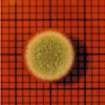
Examine the picture of the mold colony (Day 6 of Figure 1.14) and answer the question, “Where is the growth?” You will find the answer to be a fundamental component of the process.

In our language, a mathematical model is a concise verbal description of the interactions and forces that cause change with time or position of a biological system (or physical or economic or other system). The modeling process begins with a clear verbal statement based on the scientist’s understanding of the interactions and forces that govern change in the system. In order for mathematical techniques to assist in understanding the system, the verbal statement must be translated into an equation, called the dynamic equation of the model. Knowledge of the initial state of a system and the dynamic equation that describes the forces of change in the system is often sufficient to forecast an observed pattern of the system. A solution equation may be derived from the dynamic equation and an initial state of the system and a graph or table of values of the solution equation may then be compared with the observed pattern of nature. The extent to which solution equation matches the pattern is a measure of the validity of the mathematical model.

Mathematical modeling is used to describe the underlying mechanisms of a large number of processes in the natural or physical or social sciences. The chart in Figure 1.1 outlines the steps

CHAPTER 1. MATHEMATICAL MODELS OF BIOLOGICAL PROCESSES

2

followed in finding a mathematical model.

Initially a scientist examines the biology of a problem, formulates a concise description, writes equations capturing the essence of the description, solves the equations, and makes predictions about the biological process. This path is marked by the bold arrows in Figure 1.1. It is seldom so simple! Almost always experimental data stimulates exchanges back and forth between a biologist and a computational scientist (mathematician, statistician, computer scientist) before a model is obtained that explains some of the biology. This additional exchange is represented by lightly marked arrows in Figure 1.1.

Biological World

Bacteria

Mathematical World

Equations Computer Programs

Biological Dynamics

Bacteria Grow

Biologist

Observations Experiments

Mathematical Model

Growth rate depends on bacterial density, available nutrients.

I T

Dynamic equations

B t+ i — B t = R x B t

IT

I T

Measurements, Data Analysis

Bacteria Density vs Time

Solution Equations

B t = (1 + RfBo

Figure 1.1: Biology – Mathematics: Information flow chart for bacteria growth.

An initial approach to modeling may follow the bold arrows in Figure 1.1. For V. natriegens growth the steps might be:

The scientist ‘knows’ that 25% of the bacteria divide every 20 minutes.

CHAPTER 1. MATHEMATICAL MODELS OF BIOLOGICAL PROCESSES

3

• If so, then bacteria increase, B t+1 — B t , should be 0.25 B t where t marks time in 20-minute intervals and B t is the amount of bacteria at the end of the tth 20-minute interval.

• From B t+ i — B t = 0.25 B t , the scientist may conclude that

£( = 1.25*50

(More about this conclusion later).

• The scientist uses this last equation to predict what bacteria density will be during an experiment in which V. natriegens, initially at 10 6 cells per milliliter, are grown in a flask for two hours.

• In the final stage, an experiment is carried out to grow the bacteria, their density is measured at selected times, and a comparison is made between observed densities and those predicted by equations.

Reality usually strikes at this stage, for the observed densities may not match the predicted densities. If so, the additional network of lightly marked arrows of the chart is implemented.

• Adjustments to a model of V. natriegen growth that may be needed include:

1. Different growth rate: A simple adjustment may be that only, say 20%, of the bacteria are dividing every 20 minutes and B t = 1.2* B 0 matches experimental observations.

2. Variable growth rate: A more complex adjustment may be that initially 25% of the bacteria were dividing every 20 minutes but as the bacteria became more dense the growth rate fell to, say only 10% dividing during the last 20 minutes of the experiment.

3. Age dependent growth rate: A different adjustment may be required if initially all of the bacteria were from newly divided cells so that, for example, most of them grow without division during the first two 20-minute periods, and then divide during the third 20-minute interval.

4. Synchronous growth: A relatively easy adjustment may account for the fact that bacterial cell division is sometimes regulated by the photo period, causing all the bacteria to divide at a certain time of day. The green alga Chlamydomonas moewussi, for example, when grown in a laboratory with alternate 12 hour intervals of light and dark, accumulate nuclear subdivisions and each cell divides into eight cells at dawn of each day 1 .

1.1 Experimental data, bacterial growth.

Population growth was historically one of the first concepts to be explored in mathematical biology and it continues to be of central importance. Thomas Malthus in 1821 asserted a theory

“that human population tends to increase at a faster rate than its means of subsistence and that unless it is checked by moral restraint or disaster (as disease, famine, or war) widespread poverty and degradation inevitably result.” 2

iEmil Bernstein, Science 131 (1960), 1528.

CHAPTER 1. MATHEMATICAL MODELS OF BIOLOGICAL PROCESSES

4

In doing so he was following the bold arrows in Figure 1.1. World population has increased approximately six fold since Malthus’ dire warning, and adjustments using the additional network of the chart are still being argued.

Duane Nykamp of the University of Minnesota is writing Math Insight, http://mathinsight.org, a collection of web pages and applets designed to shed light on concepts underlying a few topics in mathematics. One of the pages,

http://mathinsight.org/bacterial_growth_initial_model, is an excellent display of the material of this section.

Bacterial growth data from a V. natriegens experiment are shown in Table 1.1. The population was grown in a commonly used nutrient growth medium, but the pH of the medium was adjusted to be pH 6.25 3 .

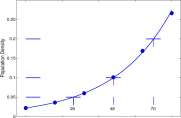
Table 1.1: Measurements of bacterial density. The units of “Population Density” are those of ab-sorbance as measured by the spectrophotometer.

How do you measure bacteria density? Ideally you would place, say 1 microliter, of growth medium under a microscope slide and count the bacteria in it. This is difficult, so the procedure commonly used is to pass a beam of light through a sample of growth medium and measure the amount of light absorbed. The greater the bacterial density the more light that is absorbed and thus bacterial density is measured in terms of absorbance units. The instrument used to do this is called a spectrophotometer.

The spectrophotometer gives you a measure of light absorbance which is directly proportional to the bacterial density (that is, light absorbance is a constant times bacterial density). Absorbance is actually defined by

Absorbance = — log 10

3 The experiment was a semester project of Deb Christensen in which several V. natriegens populations were grown in a range of pH values.

CHAPTER 1. MATHEMATICAL MODELS OF BIOLOGICAL PROCESSES

5

where Jo is the light intensity passing through the medium with no bacteria present and I t is the light intensity passing through the medium with bacteria at time t. It may seem more natural to use

Io-h Io

as a measure of absorbance. The reason for using log 10 ^ is related to our next example for light absorbance below the surface of a lake, but is only easy to explain after continuous models are studied . See Chapter ?? (Exercise ??).

1.1.1 Steps towards building a mathematical model.

This section illustrates one possible sequence of steps leading to a mathematical model of bacterial growth.

Step 1. Preliminary Mathematical Model: Description of bacterial growth.

Bacterial populations increase rapidly when grown at low bacterial densities in abundant nutrient. The population increase is due to binary fission – single cells divide asexually into two cells, subsequently the two cells divide to form four cells, and so on. The time required for a cell to mature and divide is approximately the same for any two cells.

Step 2. Notation. The first step towards building equations for a mathematical model is an introduction of notation. In this case the data involve time and bacterial density, and it is easy to let t denote time and B t denote bacterial density at time t. However, the data was read in multiples of 16 minutes, and it will help our notation to rescale time so that t is 0, 1, 2, 3, 4, or 5. Thus B3 is the bacterial density at time 3 x 16 = 48 minutes. The rescaled time is shown under ‘Time Index’ in Table 1.1.

Step 3. Derive a dynamic equation. In some cases your mathematical model will be sufficiently explicit that you are able to write the dynamic equation directly from the model. For this development, we first look at supplemental computations and graphs of the data.

Step 3a. Computation of rates of change from the data. Table 1.1 contains a computed column, ‘Population Change per Unit Time’. In the Mathematical Model, the time for a cell to mature and divide is approximately constant, and the overall population change per unit time should provide useful information.

Explore 1.1.1 Do this. It is important. Suppose the time for a cell to mature and divide is r minutes. What fraction of the cells should divide each minute? h

Using our notation,

B 0 = 0.022, B x = 0.036, B 2 = 0.060, etc.

and

B x – B 0 = 0.014, B 2 -B x = 0.024, etc.

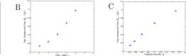
Step 3b. Graphs of the Data. Another important step in modeling is to obtain a visual image of the data. Shown in Figure 1.2 are three graphs that illustrate bacterial growth. Bacterial Growth A is a plot of column 3 vs column 2, B is a plot of column 4 vs column 2, and C is a plot of column 4 vs column 3 from the Table 1.1.

CHAPTER 1. MATHEMATICAL MODELS OF BIOLOGICAL PROCESSES

6

A

Figure 1.2: (A) Bacterial population density, B t , vs time index, t. (B) Population density change per unit time, B t+ \ — B t , vs time index, t. (C) Population density change per unit time, B t+ i — B t , vs population density, B t .

Note: In plotting data, the expression ‘plot B vs A 1 means that B is the vertical coordinate and A is the horizontal coordinate. Students sometimes reverse the axes, and disrupt a commonly used convention that began some 350 years ago. In plotting bacterial density vs time, students may put bacterial density on the horizontal axis and time on the vertical axis, contrary to widely used practice. Perhaps if the mathematician who introduced analytic geometry, Rene DesCartes of France and Belgium, had lived in China where documents are read from top to bottom by columns and from right to left, plotting of data would follow another convention.

We suggest that you use the established convention.

The graph Bacterial Growth A is a classic picture of low density growth with the graph curving upward indicating an increasing growth rate. Observe from Bacterial Growth B that the rate of growth (column 4, vertical scale) is increasing with time.

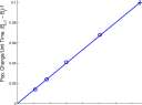
The graph Bacterial Growth C is an important graph for us, for it relates the bacterial increase to bacterial density, and bacterial increase is based on the cell division described in our mathematical model. Because the points lie approximately on a straight line it is easy to get an equation descriptive of this relation. Note: See Explore 1.1.1.

Step Sc. An Equation Descriptive of the Data. Shown in Figure 1.3 is a reproduction of the graph Bacterial Growth C in which the point (0.15,0.1) is marked with an ‘+’ and a line is drawn through (0,0) and (0.15,0.1). The slope of the line is 2/3. The line is ‘fit by eye’ to the first four points. The line can be ‘fit’ more quantitatively, but it is not necessary to do so at this stage.

Explore 1.1.2 Do this. A. Why should the line in Figure 1.3 pass through (0,0)?

B. Suppose the slope of the line is 2/3. Estimate the time required for a cell to mature and divide. m

The fifth point, which is (B4, B 5 — £> 4 ) = (0.169,0.097) lies below the line. Because the line is so close to the first four points, there is a suggestion that during the fourth time period, the growth, B 5 — £?4 = 0.97, is below expectation, or perhaps, B$ = 0.266 is a measurement error and should be larger. These bacteria were actually grown and measured for 160 minutes and we will find in Volume II, Chapter 14 that the measured value B 5 = 0.266 is consistent with the remaining data. The bacterial growth is slowing down after t = 4, or after 64 minutes.

CHAPTER 1. MATHEMATICAL MODELS OF BIOLOGICAL PROCESSES

7

o

Population Density, B (

Figure 1.3: A line fit to the first four data points of bacterial growth. The line contains (0,0) and (0.15, 0.1) and has slope = 2/3.

The slope of the line in Bacterial Growth C is = | and the ^-intercept is 0. Therefore an equation of the line is

2

y = -x y 3

Step 3d. Convert data equation to a dynamic equation. The points in Bacterial Growth C were plotted by letting x = B t and y = B t+ i — B t for t = 0, 1, 2, 3, and 4. If we substitute for x and y into the data equation y = |x we get

B t+l -B t = 2 -B t (1.1)

Equation 1.1 is our first instance of a dynamic equation descriptive of a biological process.

Step 4. Enhance the preliminary mathematical model of Step 1. The preliminary mathematical model in Step 1 describes microscopic cell division and can be expanded to describe the macroscopic cell density that was observed in the experiment. One might extrapolate from the original statement, but the observed data guides the development.

In words Equation 1.1 says that the growth during the i-th time interval is | times B t , the bacteria present at time t, the beginning of the period. The number | is called the relative growth rate – the growth per time interval is two-thirds of the current population size. More generally, one may say:

Mathematical Model 1.1.1 Bacterial Growth. A fixed fraction of cells divide every time period. (In this instance, two-thirds of the cells divide every 16 minutes.)

Step 5. Compute a solution to the dynamic equation. We first compute estimates of B\ and B2 predicted by the dynamic equation. The dynamic equation 1.1 specifies the change in bacterial density (B t+ i — B t ) from t to time t + 1. In order to be useful, an initial value of B 0 is required. We assume the original data point, B 0 = 0.022 as our reference point. It will be convenient to change B t+ i — B t = \B t into what we call an iteration equation:

2 5 Bt+i — B t = -B t B t+ i = -B t (1.2)

Iteration Equation 1.2 is shorthand for at least five equations

5 5 5 5 5

CHAPTER 1. MATHEMATICAL MODELS OF BIOLOGICAL PROCESSES

8

Beginning with B 0 = 0.022 we can compute

B l = | S 0 = §0.022 = 0.037

B 2 = | Si = §0.037 = 0.061 Explore 1.1.3 Use B 0 = 0.022 and B t+1 — § B t to compute Si, S 2 , S 3 , S 4 , and S 5 .

There is also some important notation used to describe the values of B t determined by the

iteration B t+1 = |S t . We can write

r> 5 / 5 n \ 5 5 d

^2-3 {3 &0) – 3 3 ^0

D 5 I 5 5 n I _ 5 5 5 r?

^3 – 3 U 3-°°/ – 3 3 3^0

>0

Explore 1.1.4 Write an equation for S 4 in terms of S 0 , using the pattern of the last equations. At time interval 5, we get

5 5 5 5 5 5 3 3 3 3 3 0

which is cumbersome and is usually written

Br,= [I]’ B 0 .

The general form is

5\* „ „ /5^*

B t = [ – ) S 0 = S 0 ( – ) (1.3)

Using the starting population density, S 0 = 0.022, Equation 1.3 becomes

5x t

B t = 0.022 y (1.4) and is the solution to the initial condition and dynamic equation 1.1

S 0 = 0.022, S f+ i – S t = S t

Populations whose growth is described by an equation of the form

P t = P 0 R l with R > 1

are said to exhibit exponential growth.

Equation 1.4 is written in terms of the time index, t. In terms of time, T in minutes, T = lQt and Equation 1.4 may be written

/5\T/16

B T = 0.022 I-J = 0.022 1.032 T (1.5)

Step 6. Compare predictions from the Mathematical Model with the original data.

How well did we do? That is, how well do the computed values of bacterial density, B t , match the observed values? The original and computed values are shown in Figure 1.4.

CHAPTER 1. MATHEMATICAL MODELS OF BIOLOGICAL PROCESSES

9

Figure 1.4: Tabular and graphical comparison of actual bacterial densities (o) with bacterial densities computed from Equation 1.3 (+).

The computed values match the observed values closely except for the last measurement where the observed value is less than the value predicted from the mathematical model. The effect of cell crowding or environmental contamination or age of cells is beginning to appear after an hour of the experiment and the model does not take this into account. We will return to this population with data for the next 80 minutes of growth in Section 15.6.1 and will develop a new model that will account for decreasing rate of growth as the population size increases.

1.1.2 Concerning the validity of a model.

We have used the population model once and found that it matches the data rather well. The validity of a model, however, is only established after multiple uses in many laboratories and critical examination of the forces and interactions that lead to the model equations. Models evolve as knowledge accumulates. Mankind’s model of the universe has evolved from the belief that Earth is the center of the universe, to the Copernican model that the sun is the center of the universe, to the realization that the sun is but a single star among some 200 billion in a galaxy, to the surprisingly recent realization (Hubble, 1923) that our Milky Way galaxy is but a single galaxy among an enormous universe of galaxies.

It is fortunate that our solution equation matched the data, but it must be acknowledged that two crucial parameters, P$ and r, were computed from the data, so that a fit may not be a great surprise. Other equations also match the data. The parabola, y = 0.0236 + .000186t + 0.00893t 2 , computed by least squares fit to the first five data points is shown in Figure 1.5, and it matches the data as well as does P t = 0.022(5/3)*. We prefer P t = 0.022(5/3)* as an explanation of the data over the parabola obtained by the method of least squares because it is derived from an understanding of bacterial growth as described by the model whereas the parabolic equation is simply a match of equation to data.

Exercises for Section 1.1, Experimental data, bacterial growth

CHAPTER 1. MATHEMATICAL MODELS OF BIOLOGICAL PROCESSES

10

Time – Index, t

Figure 1.5: A graph of y = 0.0236 + .000186* + 0.00893t 2 (+) which is the quadratic fit by least squares to the first six data points (o) of V. natriegens growth in Table 1.1

Exercise 1.1.1 Compute Bi, B 2 , and B 3 as in Step 5 of this section for

Exercise 1.1.2 Write a solution equation for the initial conditions and dynamic equations of Exercise 1.1.1 similar to the solution Equation 1.4, B t = (5/3)*0.022 of the pair B 0 = 0.022, B t+1 -B t = (2/3)B t .

Exercise 1.1.3 Observe that the graph Bacterial Growth C is a plot of B t+ i — B t vs B t . The points are (B 0 ,Bx — B 0 ), (B 1 ,B 2 — -Bi), etc. The second coordinate, B t+1 — B t is the population increase during time period t, given that the population at the beginning of the time period is B t . Explain why the point (0,0) would be a point of this graph.

Exercise 1.1.4 In Table 1.2 are given four sets of data. For each data set, find a number r so that the values Bi, B 2 , B 3 , B^, B 5 and B 6 computed from the difference equation

B 0 = as given in the table, B t+1 — B t = r B t

are close to the corresponding numbers in the table. Compute the numbers, B\ to Bq using your value of r in the equation, B t +i = (1 + r) B t , and compare your computed numbers with the original data.

For each data set, follow steps 3, 5, and 6. The line you draw close to the data in step 3 should go through (0,0).

Exercise 1.1.5 The bacterium V. natriegens was also grown in a growth medium with pH of 7.85. Data for that experiment is shown in Table 1.3. Repeat the analysis in steps 1 – 9 of this section for this data. After completing the steps 1-9, compare your computed relative growth rate of V. natriegens at pH 7.85 with our computed relative growth rate of 2/3 at pH 6.25.

Exercise 1.1.6 What initial condition and dynamic equation would describe the growth of an Escherichia coli population in a nutrient medium that had 250,000 E. coli cells per milliliter at the start of an experiment and one-fourth of the cells divided every 30 minutes.

CHAPTER 1. MATHEMATICAL MODELS OF BIOLOGICAL PROCESSES

11

Table 1.2: Tables of data for Exercise 1.1.4

(c)

(d)

Table 1.3: Data for Exercise 1.1.5, V. natriegens growth in a medium with pH of 7.85.

1.2 Solution to the dynamic equation P t+ \ — P t = r P t . The dynamic equation with initial condition, P 0 ,

P t+ i — P t = r P t) t — 0,1, • • •, P 0 a known value

1.6)

arises in many models of elementary biological processes. A solution to the dynamic equation 1.6 is a formula for computing P t in terms of t and Pq.

Assume that r ^0 and Po ^ 0. The equation P t+ i — P t = r P t can be changed to iteration form

by

Pt+i-Pt = rP t

P t+ i = (r + l)P t

Pt+i — RPt

(1.7)

CHAPTER 1. MATHEMATICAL MODELS OF BIOLOGICAL PROCESSES

12

number of equations, as in

Pi

P2

RP 1

t = 0 t = 1

Pn-l

RPn-2 RPn-1

t = n-2 t = n-l

where n can be any stopping value.

Cascading equations. These equations (1.8) may be ‘cascaded’ as follows.

1. The product of all the numbers on the left sides of Equations 1.8 is equal to the product of all of the numbers on the right sides. Therefore

P 1 x P 2 x • • • x P n _x x P n = RP 0 xRP ± x—x RP n -2 x R P n _i

2. The previous equation may be rearranged to

Pi P 2 ■ ■ ■ P n -i Pn — R n Po Pi ‘ ‘ ‘ Pfi-2 Pn-l-

3. Pi, P2, ■ ■ ■ P n -i are factors on both sides of the equation and (assuming no one of them is zero) may be divided from both sides of the equation, leaving

R n P 0

Because n is arbitrary and the dynamic equation is written with t, we write

p t = J R*p 0 = p 0 (i+ r y (1.9)

as the solution to the iteration

P t+ i — RP t with initial value, P 0

and the solution to

P t+ i — P t = r P t with initial value, P$.

Explore 1.2.1 a. Suppose r = 0 in P t+1 – P t = r P t so that P t+1 – P t = 0. What are P 1 , P 2 , ■ ■ •? b. Suppose P 0 = 0, and P t+1 – P t = r P t for t = 0,1, 2, • • •. What are Pi, P 2 , • • •? ■

Example 1.2.1 Suppose a human population is growing at 1% per year and initially has 1,000,000 individuals. Let P t denote the populations size t years after the initial population of Po = 1, 000, 000 individuals. If one asks what the population will be in 50 years there are two options. Option 1. At 1% per year growth, the dynamic equation would be

p t+1 -p = o.oip

and the corresponding iteration equation is

p m = i.oip

CHAPTER 1. MATHEMATICAL MODELS OF BIOLOGICAL PROCESSES

13

With P 0 = l, 000, 000, P 1 = 1.01 x 1, 000, 000 = 1, 010, 000, P 2 = 1.01 1, 010, 000 = 1, 020,100 and so on for 50 iterations.

Option 2. Alternatively, one may write the solution

P t = 1.01* (1,000,000)

so that

P 50 = 1.01 50 (1, 000, 000) = 1, 644, 631

The algebraic form of the solution, P t = R f P 0 , with r > 0 and R > 1 is informative and gives rise to the common description of exponential growth attached to some populations. If r is negative and R — 1 + r < 1, the solution equation P t = R f P 0 exhibits exponential decay.

Exercises for Section 1.2, Solution to the dynamic equation, P t+1 — P t = rP t .

Exercise 1.2.1 Write a solution equation for the following initial conditions and difference equations or iteration equations. In each case, compute -Bioo-

Exercise 1.2.2 The equation, B t — B t -i = rB t -i, carries the same information as B t+1 — B t — rB t .

a. Write the first four instances of B t — B t -\ = rB t -\ using t — 1, t — 2, t — 3, and t — 4.

b. Cascade these four equations to get an expression for _B 4 in terms of r and B 0 .

c. Write solutions to and compute -B40 for

Exercise 1.2.3 Suppose a population is initially of size 1,000,000 and grows at the rate of 2% per year. What will be the size of the population after 50 years?

Exercise 1.2.4 The polymerase chain reaction is a means of making multiple copies of a DNA segment from only a minute amounts of original DNA. The procedure consists of a sequence of, say, 30 cycles in which each segment present at the beginning of a cycle is duplicated once; at the end of the cycle that segment and one copy is present. Introduce notation and write a difference equation with initial condition from which the amount of DNA present at the end of each cycle can be computed. Suppose you begin with 1 picogram = 0.000000000001 g of DNA. How many grams of DNA would be present after 30 cycles.

CHAPTER 1. MATHEMATICAL MODELS OF BIOLOGICAL PROCESSES

14

Exercise 1.2.5 Write a solution to the dynamic equation you obtained for growth of V. natriegens in growth medium of pH 7.85 in Exercise 1.1.5. Use your solution to compute your estimate of B±.

Exercise 1.2.6 There is a suggestion that the world human population is growing exponentially.

Shown below are the human population numbers in billions of people for the decades 1940 – 2010. Year 1940 1950 1960 1970 1980 1990 2000 2010

Index, t 0 1 2 3 4 5 6 7

Human Population x 10 6 2.30 2.52 3.02 3.70 4.45 5.30 6.06 6.80

1. Test the equation

P t = 2.2 1.19*

against the data where t is the time index in decades after 1940 and P t is the human population in billions.

2. What percentage increase in human population each decade does the model for the equation assume?

3. What world human population does the equation predict for the year 2050?

1.3 Experimental data: Sunlight depletion below the surface of a lake or ocean.

Light extinction with increasing depth of water determines underwater plant, algae, and phytoplankton growth and thus has important biological consequences. We develop and analyze a mathematical model of light extinction below the surface of the ocean.

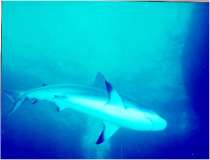
Figure 1.6: There is less light in the water below the shark than there is in the water above the shark.

Sunlight is the energy source of almost all life on Earth and its penetration into oceans and lakes largely determines the depths at which plant, algae and phytoplankton life can persist. This life is important to us: some 85% of all oxygen production on earth is by the phytoplankta diatoms and dinoflagellates 4 .

CHAPTER 1. MATHEMATICAL MODELS OF BIOLOGICAL PROCESSES

15

Explore 1.3.1 Preliminary analysis. Even in a very clear ocean, light decreases with depth below the surface, as illustrated in Figure 1.6. Think about how light would decrease if you were to descend into the ocean. Light that reaches you passes through the water column above you.

a. Suppose the light intensity at the ocean surface is Iq and at depth 10 meters the light intensity is |/ 0 – What light intensity would you expect at 20 meters?

b. Draw a candidate graph of light intensity versus depth.

We are asking you to essentially follow the bold arrows of the chart in Figure 1.7. ■

Biological World

Light, Water

Mathematical World

Equations Computer Programs

Biological Dynamics

Light Decreases with Depth

Mathematical Model

Water layers of given thickness and turbidity absorb a fixed fraction of light entering them.

I T

Biologist

Observations Experiments

Dynamic equations

It+i-It = -FI t

IT

I T

Measurements, Data Analysis

Light Intensity vs Depth

Solution Equations

I t = (1-Fflo

Figure 1.7: Biology – Mathematics: Information Flow Chart for the sunlight depletion example.

The steps in the analysis of light depletion are analogous to the steps for the analysis of bacterial growth in Section 1.1.

CHAPTER 1. MATHEMATICAL MODELS OF BIOLOGICAL PROCESSES

16

Step 1. Statement of a mathematical model. Think of the ocean as divided into layers, say one meter thick, as illustrated in Figure 1.8. As light travels downward from the surface, each layer will absorb some light. We will assume that the distribution of suspended particles in the water is uniform so that the light absorbing properties of each two layers are the same. We hypothesize that each two layers will absorb the same fraction of the light that enters it. The magnitude of the light absorbed will be greater in the top layers than in the lower layers simply because the intensity of the light entering the the top layers is greater than the intensity of light at the lower layers. We state the hypothesis as a mathematical model.

Mathematical Model 1.3.1 Light depletion with depth of water. Each layer absorbs a fraction of the light entering the layer from above. The fraction of light absorbed, f, is the same for all layers of a fixed thickness.

Surface

d

d+1

Figure 1.8: A model of the ocean partitioned into layers.

Step 2. Notation We will let d denote depth (an index measured in layers) and Id denote light intensity at depth d. Sunlight is partly reflected by the surface, and Jo (light intensity at depth 0) is to be the intensity of the light that penetrates the surface. I\ is the light intensity at the bottom of the first layer, and at the top of the second layer.

The opacity 5 of the water is due generally to suspended particles and is a measure of the turbidity of the water. In relatively clear ocean water, atomic interaction with light is largely responsible for light decay. In the bacterial experiments, the growth of the bacteria increases the turbidity of the growth serum, thus increasing the opacity and the absorbance.

The fraction, /, of light absorbed by each layer is between 0 and 1 (or possibly 1, which would not be a very interesting model). Although / is assumed to be the same for all layers, the value of / depends on the thickness of the layer and the distribution of suspended particles in the water and atomic interactions with light. Approximately,

/ = Layer thickness x Opacity of the water.

5 Wikipedia. Opacity – the degree to which light is not allowed to travel through. Turbidity- the cloudiness or haziness of a fluid caused by individual particles (suspended particles) that are generally invisible to the naked eye.

CHAPTER 1. MATHEMATICAL MODELS OF BIOLOGICAL PROCESSES

17

Layer thickness should be sufficiently thin that the preceding approximation yields a value of / substantially less than 1. We are developing a discrete model of continuous process, and need layers thin enough to give a good approximation. The continuous model is shown in Subsection 5.5.2. Thus for high opacity of a muddy lake, layer thickness of 20 cm might be required, but for a sparkling ocean, layer thickness of 10 m might be acceptable.

Explore 1.3.2 Assume that at the surface light intensity Io is 400 watts/meter-squared and that each layer of thickness 2 meters absorbs 10% of the light that enters it. Calculate the light intensity at depths 2, 4, 6, • • •, 20 meters. Plot your data and compare your graph with the graph you drew in Explore 1.3.1. ■

Step 3. Develop a dynamic equation representative of the model. Consider the layer between depths d and d + 1 in Figure 1.8. The intensity of the light entering the layer is Id-

The light absorbed by the layer between depths d and d + 1 is the difference between the light entering the layer at depth d and the light leaving the layer at depth d+1, which is Id — I d +\-

The mathematical model asserts that

I d – h+i = fh (1.10)

Note that Id decreases as d increases so that both sides of equation 1.10 are positive common to write

Id+i ~ h = —f Id and to put this equation in iteration form

I d+1 = (l-f)I d Id+i=FI d (1.12)

where F = 1 – /. Because 0 < / < 1, also 0 < F < 1.

Step 4. Enhance the mathematical model of Step 1. We are satisfied with the model of Step 1 (have not yet looked at any real data!), and do not need to make an adjustment.

Step 5. Solve the dynamical equation, I d+1 — Id — —f h- The iteration form of the dynamical equation is I d +i — F Id and is similar to the iteration equation B t+i — | B t of bacterial

growth for which the solution is B t = B 0 (|) . We conclude that the solution of the light equation is

Id = Io F d (1.13)

The solutions,

B t = B 0 (^ and I d = I 0 F d F<1

are quite different in character, however, because | > 1, (|) increases with increasing t and for F < 1, F d decreases with increasing d.

CHAPTER 1. MATHEMATICAL MODELS OF BIOLOGICAL PROCESSES

18

Step 6. Compare predictions from the model with experimental data. It is time we looked at some data. We present some data, estimate / of the model from the data, and compare values computed from Equation 1.13 with observed data.

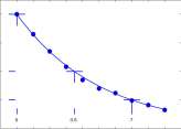
In measuring light extinction, it is easier to bring the water into a laboratory than to make measurements in a lake, and our students have done that. Students collected water from a campus lake with substantial suspended particulate matter (that is, yucky). A vertically oriented 3 foot section of 1.5 inch diameter PVC pipe was blocked at the bottom end with a clear plastic plate and a flashlight was shined into the top of the tube (see Figure 1.9). A light detector was placed below the clear plastic at the bottom of the tube. Repeatedly, 30 cm 3 of lake water was inserted into the tube and the light intensity at the bottom of the tube was measured. One such data set is given in Figure 1.9 6 .

Figure 1.9: Diagram of laboratory equipment and data obtained from a light decay experiment.

Explore 1.3.3 In Figure 1.10A is a graph of Id vs d. Compare this graph with the two that you drew in Explore 1.3.1 and 1.3.2. ■

Our dynamical equation relates Id+i ~ Id to Id and we compute change in intensity, Ij+i — Id, just as we computed changes in bacterial population. The change in intensity, Ij+i — Id, is the amount of light absorbed by layer, d.

Graphs of the data. A graph of the original data, Id vs d, is shown in Figure 1.10(A) and and a graph of I d +i — Id vs I d is shown in Figure 1.10(B).

In Figure 1.10(B) we have drawn a line close to the data that passes through (0,0). Our reason that the line should contain (0,0) is that if I d , the amount of light entering layer d is small, then I d +i — h, the amount of light absorbed by that layer is also small. Therefore, for additional layers, the data will cluster near (0,0).

The graph of Id+i — Id vs Id is a scattered in its upper portion, corresponding to low light intensities. There are two reasons for this.

1. Maintaining a constant light source during the experiment is difficult so that there is some error in the data.

6 This laboratory is described in Brian A. Keller, Shedding light on the subject, Mathematics Teacher 91 (1998), 756-771.

CHAPTER 1. MATHEMATICAL MODELS OF BIOLOGICAL PROCESSES

19

3 t 5 6 7 8 9 10

Depth — layers — d L ‘9 nt ‘”tensity — l d

Figure 1.10: (A) The light decay curve for the data of Figure 1.9 and (B) the graph of light absorbed by layers vs light entering the layer from Table 1.9.

2. Subtraction of numbers that are almost equal emphasizes the error, and in some cases the error can be as large as the difference you wish to measure. In the lower depths, the light values are all small and therefore nearly equal so that the error in the differences is a large percentage of the computed differences.

Use the data to develop a dynamic equation. The line goes through (0,0) and the point (0.4, -0.072). An equation of the line is

y = -0.18a;

Remember that y is 4+i — 4 an d x is Id and substitute to get

/ d+ i-/ d = -0.18/ d (1.14)

This is the dynamic Equation 1.11 with —/ = —0.18.

Solve the dynamic equation. (Step 5 for this data.) The iteration form of the dynamic equation is

4+1 = 4-0.184 I d+1 = 0.82I d

and the solution is (with I 0 = 0.400)

4 = 0.82 d / 0 = 0.400 0.82 d (1.15)

Compare predictions from the Mathematical Model with the original data. How

well did we do? Again we use the equations of the model to compute values and compare them with the original data. Shown in Figure 1.11 are the original data and data computed with Id = 0.400 0.82 d , and a graph comparing them.

The computed data match the observed data quite well, despite the ‘fuzziness’ of the graph in Figure 1.10(b) of 4+i ~~ 4 vs Id from which the dynamic equation was obtained.

Exercises for Section 1.3, Experimental data: Sunlight depletion below the surface of a

lake or ocean.

CHAPTER 1. MATHEMATICAL MODELS OF BIOLOGICAL PROCESSES

20

Figure 1.11: Comparison of original light intensities (o) with those computed from I d = 0.82 d 0.400 (+)•

Exercise 1.3.1 In Table 1.4 are given four sets of data that mimic light decay with depth. For each data set, find a number r so that the values B 1 , B 2 , B 3 , B±, B 5 and B G computed from the difference equation

Bq = as given in the table, B t +\ — B t = —r B t

are close to the corresponding numbers in the table. Compute the numbers, B\ to Bq using your value of R in the equation and compare your computed numbers with the original data.

For each data set, follow steps 3, 5, and 6. The line you draw close to the data in step 3 should go through (0,0).

Table 1.4: Tables of data for Exercise 1.3.1

(d)

Exercise 1.3.2 Now it is your turn. Shown in the Exercise Table 1.3.2 are data from a light experiment using the laboratory procedure of this section. The only difference is the water that was used. Plot the data, compute differences and obtain a dynamic equation from the plot of differences vs intensities. Solve the dynamic equation and compute estimated values from the

CHAPTER 1. MATHEMATICAL MODELS OF BIOLOGICAL PROCESSES

21

intensities and compare them with the observed light intensities. Finally, decide whether the water from your experiment is more clear or less clear than the water in Figure 1.9. (Note: Layer thickness was the same in both experiments.)

Table for Exercise 1.3.2 Data for Exercise 1.3.2.

Depth Layer 012345678 Light Intensity 0.842 0.639 0.459 0.348 0.263 0.202 .154 0.114 0.085

Exercise 1.3.3 One might reasonably conclude that the graph in Figure 1.10(a) looks like a parabola. Find an equation of a parabola close to the graph in Figure 1.10(a). Your calculator may have a program that fits quadratic functions to data, or you may run the MATLAB program:

close all;clc;clear D=[0:l:9] ;

I=[0.4 0.33 0.27 0.216 0.17 0.14 0.124 0.098 0.082 0.065];

P=polyfit(D,I,2)

X=[0:0.1:9]; Y=polyval(P,X);

plot(D,I,’o’,’linewidth’,2);

hold(‘on’);

plot(X,Y,’linewidth’,2)

The structure of a program to fit a parabola to data is:

1. Close and clear all previous graphs and variables. [Perhaps unnecessary]

2. Load the data. [In lists D (depths) and I (light intensity)].

3. Compute the coefficients of a second degree polynomial close to the data and store them in P.

4. Specify X coordinates for the polynomial and compute the corresponding Y coordinates of the polynomial.

5. Plot the original data as points.

6. Plot the computed polynomial.

Compare the fit of the parabola to the data in Figure 1.10(a) with the fit of the graph of I a = 0.400 0.82 d to the same data illustrated in Figure 1.11.

The parabola fits the data quite well. Why might you prefer I d = 0.400 0.82 d over the equation of the parabola as an explanation of the data?

Exercise 1.3.4 A light meter suitable for underwater photography was used to measure light intensity in the ocean at Roatan, Honduras. The meter was pointed horizontally. Film speed was set at 400 ASA and time at 1/60 s. The recommended shutter apertures (/stop) at indicated depths are shown in Table Ex. 1.3.4. We show below that the light intensity is proportional to the square of the recommended shutter aperture. Do the data show exponential decay of light?

Notes. The quanta of light required to expose the 400 ASA film is a constant, C. The amount of light that strikes the film in one exposure is A AT I, where A is area of shutter opening, AT is the time of exposure (set to be 1/60 s) and / is light intensity (quanta/(cm 2 -sec)). Therefore

C = AATxI or / = C-^—\ = 600^

CHAPTER 1. MATHEMATICAL MODELS OF BIOLOGICAL PROCESSES

22

By definition of /-stop, for a lense of focal length, F, the diameter of the shutter opening is F/(/-stop) mm. Therefore

The last two equations yield

/ = 60(^-^2 (/-stop) 2 = K(f-stop) 2 where K = 60C-^. Thus light intensity, I is proportional to (/-stop) 2 .

Table for Exercise 1.3.4 /-stop specifications for 400 ASA film at 1/60 s exposure at various depths below the surface of the ocean near Roatan, Honduras.

1.4 Doubling Time and Half-Life.

Populations whose growth can be described by an exponential function (such as

Pop = 0.022 1.032 T ) have a characteristic doubling time, the time required for the population to

double. The graph of the V. natriegens data and the graph of P = 0.022 1.032 T (Equation 1.5) that

we derived from that data is shown in Figure 1.12. See Also:

http: //mathinsight.org/doubling_time_half _life_discrete

0 20 40 60 80

Time – Min

Figure 1.12: Data for V. natriegens growth and the graph of P = 0.022 1.032 T .

Observe that at T = 26, P = 0.05 and at T = 48, P = 0.1; thus P doubled from 0.05 to 0.1 in the 22 minutes between T = 26 and T = 48. Also, at T = 70, P = 0.2 so the population also doubled from 0.1 to 0.2 between T = 48 and T = 70, which is also 22 minutes.

CHAPTER 1. MATHEMATICAL MODELS OF BIOLOGICAL PROCESSES

23

The doubling time, T Doub i c , can be computed as follows for exponential growth of the form

P = A B l B>1

Let Pi be the population at any time T\ and let T 2 be the time at which the population is twice Pi. The doubling time, Tnoubie, is by definition T 2 — T\ and

Pi = A B Tl and

Therefore

2 A B Tl =

2 = 2 =

^Double = T2 — T\ =

Thus the doubling time for the equation P only on B and not on A nor on the base of the logarithm.

For the equation, Pop = 0.022 1.032 T , the doubling time is log 2/log 1.032 = 22.0056, as shown in the graph.

Half Life. For the exponential equation y = A B T with B < 1, y does not grow. Instead, y decreases. The half-life, Tn a if, of y is the time it takes for y to one-half it initial size. The word, ‘half-life’ is also used in the context y = A B x where x denotes distance instead of time.

Data for light extinction below the surface of a lake from Section 1.3 on page 14 is shown in Figure 1.13 together with the graph of

I d = 0.4 0.82 d

Horizontal segments at Light = 0.4, Light = 0.2, and Light = 0.1 cross the curve in Figure 1.13 at d = 0, d = 3.5 and d = 7. The ‘half-life’ of the light is 3.5 layers of water.

0.3

■f 1

JE 0.2

-1 01 23456789 10

Depth — layers

Figure 1.13: Graph of light intensity with depth and the curve I d = 0.4 0.82 d .

P T = 2 Pi = A B T2

A B T ‘ 2

B^

B T2 ~ Tl

—-— Doubling Time (1-16) logP

= AB T is log 2/log P. The doubling time depends

CHAPTER 1. MATHEMATICAL MODELS OF BIOLOGICAL PROCESSES

24

It might make more sense to you to call the number 3.5 the ‘half-depth’ of the light, but you will be understood by a wider audience if you call it ‘half-life’.

In Exercise 1.4.9 you are asked to prove that the half-life, T Ha if, of

y = A B T , where B < 1 is

^Half

log

1 (1-17)

2 _ – log 2

Iog~B log B

Exercises for Section 1.4 Doubling Time and Half-Life.

Exercise 1.4.1 Determine the doubling times of the following exponential equations.

(a) y = 2* (b) y = 2 3t (c) y = 2 0At

(d) y = 10* (e) y = 10 3t (f) y = 10 01 *

Exercise 1.4.2 Show that the doubling time of y = A B l is l/(log 2 B).

Exercise 1.4.3 Show that the doubling time of y = A 2 kt is 1/k.

Exercise 1.4.4 Determine the doubling times or half-lives of the following exponential equations.

(a) y = 0.5* (b) y = 2 3t (c) y = 0A 0At

(d) y = 100 0.8* (e) y = 45 3i (f) y = 0.0001 5 ai *

(g) y = 10 0.8 2 * (h) y = 0.01 3 * (i) y = 0.01 ai *

Exercise 1.4.5 Find a formula for a population that grows exponentially and

a. Has an initial population of 50 and a doubling time of 10 years.

b. Has an initial population of 1000 and a doubling time of 50 years.

c. Has in initial population of 1000 and a doubling time of 100 years.

Exercise 1.4.6 An investment of amount A 0 dollars that accumulates interest at a rate r compounded annually is worth

A t = A 0 (i + r y

dollars t years after the initial investment.

a. Find the value of A w if A 0 — 1 and r = 0.06.

b. For what value of r will A 8 = 2 if A 0 = 1?

c. Investment advisers sometimes speak of the “Rule of 72”, which asserts that an investment at R percent interest will double in 72/R years. Check the Rule of 72 for R = 4, R = 6,

R = 8, R = 9 and R = 12.

Exercise 1.4.7 Light intensities, I\ and J 2 , are measured at depths d in meters in two lakes on two different days and found to be approximately

CHAPTER 1. MATHEMATICAL MODELS OF BIOLOGICAL PROCESSES

25

a. What is the half-life of /]?

b. What is the half-life of J 2 ?

c. Find a depth at which the two light intensities are the same.

d. Which of the two lakes is the muddiest?

Exercise 1.4.8 a. The mass of a single V. natriegens bacterial cell is approximately 2 1CT 11 grams. If at time 0 there are 10 8 V. natriegens cells in your culture, what is the mass of bacteria in your culture at time 0?

b. We found the doubling time for V. natriegen to be 22 minutes. Assume for simplicity that the doubling time is 30 minutes and that the bacteria continue to divide at the same rate. How may minutes will it take to have a mass of bacteria from Part a. equal one gram?

c. The earth weighs 6 10 27 grams. How many minutes will it take to have a mass of bacteria equal to the mass of the Earth? How many hours is this? Why aren’t we worried about this in the laboratory? Why hasn’t this happened already in nature? Explain why it is not a good idea to extrapolate results far beyond the end-point of data gathering.

Exercise 1.4.9 Show that y = A B t with B < 1 has a half-life of

T = ]°sl = -^g 2

log B log-B ‘

1.5 Quadratic Solution Equations: Mold growth

We examine mold growing on a solution of tea and sugar and find that models of this process lead to quadratic solution equations in contrast to the previous mathematical models which have exponential solution equations. Quadratic solution equations (equations of the form y = at 2 + bt + c) occur less frequently than do exponential solution equations in models of biological systems.

Shown in Figure 1.14 are some pictures taken of a mold colony growing on the surface of a mixture of tea and sugar. The pictures were taken at 10:00 each morning for 10 consecutive days. Assume that the area occupied by the mold is a reasonable measure of the size of the mold population. The grid lines are at 2mm intervals.

Explore 1.5.1 From the pictures, measure the areas of the mold for the days 2 and 6 and enter them into the table of Figure 1.15. The grid lines are at 2mm intervals, so that each square is 4mm 2 . Check your additional data with points on the graph. ■

CHAPTER 1. MATHEMATICAL MODELS OF BIOLOGICAL PROCESSES

26

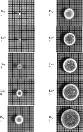
Figure 1.14: Pictures of a mold colony, taken on ten successive days. The grid lines are at 2mm intervals.

CHAPTER 1. MATHEMATICAL MODELS OF BIOLOGICAL PROCESSES

27

Time – days

Figure 1.15: Areas of the mold colonies shown in Figure 1.14

Explore 1.5.2 Do this. It is interesting and important to the remaining analysis. Find numbers A and B so that the graph of y = AlB 1 approximates the mold growth data in Figure 1.14. Either chose two data points and insist that the points satisfy the equation or use a calculator or computer to compute the least squares approximation to the data. Similarly find a parabola y = at 2 + bt + c that approximates the mold data. Draw graphs of the mold data, the exponential function, and the parabola that you found on a single set of axes. ■

Many people would expect the mold growth to be similar to bacterial growth and to have an exponential solution equation. We wish to explore the dynamics of mold growth.

Step 1. Mathematical model. Look carefully at the pictures in Figure 1.14. Observe that the features of the interior dark areas, once established, do not change. The growth is restricted to the perimeter of the colony 7 . On this basis we propose the model

Mathematical Model 1.5.1 Mold growth. Each day the increase in area of the colony is proportional to the length of the perimeter of the colony at the beginning of the day (when the photograph was taken).

Step 2. Notation. We will let t denote day of the experiment, A t the area of the colony and C t the length of the colony perimeter at the beginning of day t.

Step 3. Dynamic equation. The statement that ‘a variable A is proportional to a variable B’ means that there is a constant, k, and

A = k B

Thus, ‘the increase in area of the colony is proportional to the perimeter’ means that there is a constant, k, such that

increase in area = k perimeter

The increase in the area of the colony on day t is A t+ i — A t , the area at the beginning of day t + 1 minus the area at the beginning of day t. We therefore write

A t+1 -A t = kC t

7 The pictures show the mold colony from above and we are implicitly taking the area of the colony as a measure of the colony size. There could be some cell division on the underside of the colony that would not be accounted for by the area. Such was not apparent from visual inspection during growth as a clear gelatinous layer developed on the underside of the colony.

CHAPTER 1. MATHEMATICAL MODELS OF BIOLOGICAL PROCESSES

28

We now make the assumption that the mold colony is circular, so that 8

C t = 2v^ Therefore

A t+ i -A t — k 2y/7T^At (1.18)

Step 5. Solve the dynamic equation. The dynamic equation 1.18 is difficult to solve, and may not have a useful formula for its solution 9 . The formula, A t = 0, defines a solution that is not useful. (Exercise 1.5.2).

A similar dynamic equation

A t+1 – A t ^ = K\J~A t (1.19)

has a solution

At = ^ (1.20)

and we ask you to confirm this solution in Exercise 1.5.5. The solution A t = ^-t 2 has A 0 = 0, which is not entirely satisfactory. (There was no mold on day 0.)

You are asked in Exercise 1.5.4 to estimate k l^n of Equation 1.18 and to iteratively compute approximations to A 0 , ■ ■ ■ Ag.

The difficulties at this stage lead us to reconsider the original problem.

Step 4. Reformulate the mathematical model. We have assumed the mold colony to be a circle expanding at its edges. We suggest that the radius is increasing at a constant rate, and write the following model.

Step 1. Mold growth, reformulated. Each day the radius of the colony increases by a constant amount.

Step 2. Notation, again. Let p t be the radius 10 of the colony at the beginning of day t, and let A (Greek letter delta) denote constant daily increase in radius.

Step 3. Dynamic equation, again. The increase in radius on day t is p t+ \ — pt, the radius at the beginning of day t + 1 minus the radius at the beginning of day t, and we write

pt+i — pt — A (1.21)

An important procedure in developing equations is to write a single thing two different ways, as we have just done for the increase in radius. Indeed, most equations do write a single thing two different ways.

You should check that the dimensions of the quantities on both sides of your equation are identical. This may assist in identifying dimensions of parameters in your equation.

8 For a circle of radius r,

Area: A = irr 2 , r — y/A/n, Circumference: C — 2nr = 2t\\] A/it =

9 We spare you the details, but it can be shown that there is neither a quadratic nor exponential solution to Equation 1.18

CHAPTER 1. MATHEMATICAL MODELS OF BIOLOGICAL PROCESSES

29

Step 4. Solution equation, again. Convert p t+ \ — p t = A to p t+ \ = p t + A and write

pi = p 0 + A, p 2 = pi + A

(p 0 + A) + A = po + 2A

and correctly guess that

Pt = p 0 + tA (1.22) Evaluate po and A. From A t = irpj, p t = JA t /ir, and

po = \/A 0 /n = ^4/^= 1.13 p 9 = \J A$ /tx = ^420/tt = 11.56

There are 9 intervening days between measurements po and pg so the average daily increase in radius is

11.56-1.13

A = = 1.16

9

We therefore write (po = 1.13, A = 1.16)

p t = 1.13 + t 1.16

Now from A t = irpf we write

A t = tt (1.13 + 1.16t) 2 (1.23)

Step 6. Compare predictions from the model with observed data. A graph of A t = it (1.13 + 1.164) and the original mold areas is shown in Figure 1.16 where we can see a reasonable fit, but there is a particularly close match at the two end points. It may be observed that only those two data points enter into calculations of the parameters 1.13 and 1.16 of the solution, which explains why the curve is close to them.

.O 250 –

o

o

• ^

Time – days

Figure 1.16: Comparison of the solution equation 1.23 with the actual mold growth data.

Exercises for Section 1.5, Quadratic solution equations: Mold growth.

CHAPTER 1. MATHEMATICAL MODELS OF BIOLOGICAL PROCESSES

30

Exercise 1.5.1 You will have found in Explore 1.5.2 that the data is approximated pretty well by both an exponential function and a quadratic function. Why might you prefer a quadratic function?

Exercise 1.5.2 Show that A t = 0 for all t is a solution to Equation 1.18,

A t+1 -A t = 2ixk^A t

This means that for every t, if A t = 0 and A t+1 is computed from the equation, then A t+1 = 0 (and, yes, this is simple).

Exercise 1.5.3 Use data at days 2 and 8, (2,24) and (8,326), to evaluate A and po in Equation 1.22

Pt = Po + t A.

See Step 4, Solution Equation, Again.

Use the new values of po and A in p t = p 0 + 1 A to compute estimates of po, pi, • • •, pg and A 0 , Ai, ■ ■ •, Ag. Plot the new estimates of A t and the observed values of A t and compare your graph with Figure 1.16.

Exercise 1.5.4 a. Compute A t+1 — A t and \[A t for the mold data in Figure 1.15 and plot A t+ \ — A t vs \fA t . You should find that the line y = 5x lies close to the data. This suggests that 5 is the value of k in Equation 1.18, A t+1 — A t = k 2^y/A~ t .

b. Use

A 0 = 4, A t+1 -A t = 5^/At

to compute estimates of Ai, • • •, Ag. Compare the estimates with the observed data.

c. Find a value of K so that the estimates computed from

A 0 = 4, A t+1 -A t = K^A t more closely approximates the observed data than do the previous approximations.

Exercise 1.5.5 Examine the following model of mold growth:

Model of mold growth, III. The increase in area of the mold colony during any time interval is proportional to the length of the circumference of the colony at the midpoint of the time interval.

A schematic of a two-day time interval is

A t -r C t

Day t _i Day t Day m

Two-day Interval

CHAPTER 1. MATHEMATICAL MODELS OF BIOLOGICAL PROCESSES

31

a. Explain the derivation of the dynamic equation

A t+1 -At-i = kC t

from Model of mold growth, III.

With C t = 2^/iTy/At = KyfA~ t , the dynamic equation becomes

A+i – A-i = K JX t

b. Show by substitution that

K 2

16

-t z

is a solution to

At+i – A

t-i

K\ A*

To do so, you will substitute A t +i — ^{t+ l) 2 , A t -\ = ^(t — l) 2 , and A t = j^t 2 , and show

that the left and right sides of the equation simplify to ^rt.

c. When you find a value for K, you will have a quadratic solution for mold growth.

In the Figure 1.17 are values of A t+1 — A t _x and \fA~ t and a plot of A t+X — A t _x vs \[A t , with one data point omitted. Compute the missing data and identify the corresponding point on the graph.

Square Root of Mold Area – A (

Figure 1.17: Data for Exercise 1.5.5, to estimate K in A t+ i — A t _i = K\[A~ t .

d. Also shown on the graph of A t+ \ — A t -\ vs \[A~ t is the graph of y = 9.15a; which is the line of the form y = mx that is closest to the data. Let K = 9.15 in A t = ^t 2 and compute A 0 , Ax, ■ ■ ■, Ag. Compare the computed values with the observed values of mold areas.

Exercise 1.5.6 Suppose a, b, and c are numbers and

P t = at 2 + bt + c

where t is any number. Show that

Qt = Pt+i ~ Pt

is linearly related to t (that is, Q t = at + (3 for some a and 0), and that

Rt = Qt+i — Qt

is a constant.

CHAPTER 1. MATHEMATICAL MODELS OF BIOLOGICAL PROCESSES

32

1.6 Constructing a Mathematical Model of Penicillin Clearance.

In this section you will build a model of depletion of penicillin from plasma in a patient who has received a bolus injection of penicillin into the plasma.

When penicillin was first discovered, its usefulness was limited by the efficiency with which the kidney eliminates penicillin from the blood plasma passing through it. “Penicillin is actively excreted, and about 80% of a penicillin dose is cleared from the body within three to four hours of administration. Indeed, during the early penicillin era, the drug was so scarce and so highly valued that it became common to collect the urine from patients being treated, so that the penicillin in the urine could be isolated and reused. 11 ” The modifications that have been made to penicillin (leading to amphicillin, moxicillin, mezlocillin, etc.) have enhanced its ability to cross membranes and reach targeted infections and reduced the rate at which the kidney clears the plasma of penicillin. Even with these improvements in penicillin, the kidneys remove 20 percent of the penicillin in the plasma passing through them. Furthermore, all of the blood plasma of a human passes through the kidneys in about 5 minutes. We therefore formulate

Mathematical Model 1.6.1 Renal clearance of penicillin. In each five minute interval following penicillin injection, the kidneys remove a fixed fraction of the penicillin that was in the plasma at the beginning of the five minute interval.

We believe the fraction to be about 0.2 so that 5 minutes after injection of penicillin into a vein, only 80% of the penicillin remains. This seems surprising and should cause you to question our assertion about renal clearance of penicillin 12 . See Also: http: //mathinsight.org/penicillin_clearance_model

An amount of drug placed instantaneously (that is, over a short period of time) in a body compartment (plasma, stomach, muscle, etc.) is referred to as a bolus injection. An alternative procedure is continuous infusion as occurs with an intravenous application of a drug. Geologists refer to a meteor entering the atmosphere as a bolide. Data for penicillin concentration following a 2 g bolus injection are shown in Figure 1.18.

Explore 1.6.1 We think you will be able to develop this model without reading our development, and will find it much more interesting than reading a solution. You have a mathematical model and relevant data. You need to

Step 2. Introduce appropriate notation.

Step 3. Write a dynamic equation describing the change in penicillin concentration. You will need a crucial negative sign here, because penicillin is removed, and the change in penicillin concentration is negative. Evaluate a parameter of the dynamic equation.

11 http://en.wikipedia.org/wiki/Penicillin, which cites Silvcrthorn, D.U., Human Physiology: An Integrated Approach (3rd Ed.) Upper Saddle River, NJ, Pearson Education

12 That all of the plasma passes through the kidney in 5 minutes is taken from Rodney A. Rhoades and George A. Tanner, Medical Physiology, Little, Brown and Company, Boston, 1995. “In resting, healthy, young adult men, renal blood flow averages about 1.2 L/min”, page 426, and “The blood volume is normally 5-6 L in men and 4.5-5.5 L in women.”, page 210. “Hematocrit values of the blood of health adults are 47 ± 5% for men and 42 ± 5% for women”, page 210 suggests that the amount of plasma in a male is about 6 L x 0.53 = 3.18 L. J. A. Webber and W. J. Wheeler, Antimicrobial and pharmacokinetic properties, in Chemistry and Biology of /3-Lactin Antibiotics, Vol. 1, Robert B. Morin and Marvin Gorman, Eds. Academic Press, New York, 1982, page 408 report plasma renal clearances of penicillin ranging from 79 to 273 ml/min. Plasma (blood minus blood cells) is approximately 53% of the blood so plasma flow through the kidney is about 6 liters x 0.53/5 min = 0.636 l/min. Clearance of 20% of the plasma yields plasma penicillin clearance of 0.636 = 0.2 = 0.127 l/min = 127 ml/min which is between 79 and 273 ml/min.

CHAPTER 1. MATHEMATICAL MODELS OF BIOLOGICAL PROCESSES

33

0 5 10 15 20

Time min

Figure 1.18: Data for serum penicillin concentrations at 5 minute intervals for the 20 minutes following a ‘bolus’ injection of 2 g into the serum of “five healthy young volunteers (read ‘medical students’)” taken from T. Bergans, Penicillins, in Antibiotics and Chemotherapy, Vol 25, H. Sch0onfeld, Ed., S. Karger, Basel, New York, 1978. We are interpreting serum in this case to be plasma.

Step 4. Review the mathematical model (it will be excellent and this step can be skipped). Step 5. Write a solution equation to the dynamic equation.

Step 6. Compare values computed with the solution equation with the observed data (you will find a very good fit).

You will find that from this data, 23 percent of the mezlocillin leaves the serum every five minutes.

Exercises for Section 1.6, Constructing a Mathematical Model of Penicillin Clearance.

Exercise 1.6.1 A one-liter flask contains one liter of distilled water and 2 g of salt. Repeatedly, 50 ml of solution are removed from the flask and discarded after which 50 ml of distilled water are added to the flask. Introduce notation and write a dynamic equation that will describe the change of salt in the beaker each cycle of removal and replacement. How much salt is in the beaker after 20 cycles of removal?

Exercise 1.6.2 A 500 milligram penicillin pill is swallowed and immediately enters the intestine. Every five minute period after ingestion of the pill

1. 10% of the penicillin in the intestine at the beginning of the period is absorbed into the plasma.

2. 15% of the penicillin in the plasma at the beginning of the period is removed by the kidney.

Let It be the amount of penicillin in the intestine and S t be the amount of penicillin in the plasma at the end of the tth five minute period after ingestion of the pill. Complete the following

CHAPTER 1. MATHEMATICAL MODELS OF BIOLOGICAL PROCESSES

34

equations, including + and – signs. Initial conditions

h = –

S 0 = .

Penicillin change Penicillin Penicillin

per time period removed added

It+i-It =

St+i — St =

Exercise 1.6.3 Along with the data for 2 gm bolus injection of mezlocillin, T. Bergan reported serum mezlocillin concentrations following 1 g bolus injection in healthy volunteers and also data following 5 g injection in healthy volunteers. Data for the first twenty minutes of each experiment are shown in Table Ex. 1.6.3.

a. Analyze the data for 1 g injection as prescribed below.

b. Analyze the data for 5 g injection as prescribed below.

Analysis. Compute P t+ \ — Pt for t — 0,1, 2, 3 and find a straight line passing through (0,0), (y = mx), close to the graph of Pt+i — Pt vs P t . Compute a solution to Pt+i — Pt = mPt, and use your solution equation to compute estimated values of Pt- Prepare a table and graph to compare your computed solution with the observed data.

Table for Exercise 1.6.3 Plasma mezlocillin concentrations at five minute intervals following injection of either 1 g of mezlocillin or 5 g of mezlocillin into healthy volunteers.

1 g injection

Mezlocillin

concentration /ig/ml

71

56 45 33 25

5 g injection

Time min

0 5 10 15 20

Time Index

Mezlocillin

concentration /ig/ml

490 390 295 232 182

Exercise 1.6.4 Two litera of fresh water (distilled H 2 0) is contained in a plastic bag that is floating in the ocean. A small area of a side of the plastic bag is a semipermeable membrane (permeable to water but not to salt). Osmosis will drive the water out of the plastic bag and into the ocean

Write a mathematical model of the transfer of water from the plastic bag to the ocean. Introduce notation and write an initial condition and a difference equation with that will describe the amount of water in the small container.

CHAPTER 1. MATHEMATICAL MODELS OF BIOLOGICAL PROCESSES

35

Exercise 1.6.5 There is a standard osmosis experiment in biology laboratory as follows.

Material: A thistle tube, a 1 liter flask, some ‘salt water’, and some pure water, a membrane that is impermeable to the salt and is permeable to the water.

The bulb of the thistle tube is filled with salt water, the membrane is placed across the open part of the bulb, and the bulb is inverted in a flask of pure water so that the top of the pure water is at the juncture of the bulb with the stem.

Because of osmotic pressure the pure water will cross the membrane pushing water up the stem of the thistle tube until the increase in pressure inside the bulb due to the water in the stem matches the osmotic pressure across the membrane.

Our problem is to describe the height of the water in the stem as a function of time. The following mathematical model would be appropriate.

Mathematical Model. The amount of water crossing the membrane during any minute is proportional to the osmotic pressure across the membrane minus the pressure due to the water in the stem at the beginning of the minute.

Assume that the volume of the bulb is much larger than the volume of the stem so that the concentration of ‘salt’ in the thistle tube may be assumed to be constant, thus making the osmotic pressure a constant, Pq (This is fortunate!). Assume that the radius of the thistle tube stem is r cm. Then an amount, V cm 3 , of additional water inside the thistle tube will cause the water to rise V/(iTr 2 ) cm. Assume the density of the salt water to be 5 gm/cm.

Introduce notation and write a difference equation with initial condition that will describe the height of the water in the stem as a function of time.

1.7 Movement toward equilibrium.

Now we consider a new mathematical model that is used to describe the response of systems to constant infusion of material or energy. Examples include

• A pristine lake has a constant flow of fresh water into it and an equal flow of water out of the lake. A factory is built next to the lake and each day releases a fixed amount of chemical waste into the lake. The chemical waste will mix through out the lake and some will leave the lake in the water flowing out. The amount of chemical waste in the lake will increase until the amount of chemical leaving the lake each day is the same as the amount released by the factory each day.

• The nitrogen in the muscle of a scuba diver is initially at 0.8 atm, the partial pressure of N 2 in atmospheric air. She descends to 20 meters and breathes air with N 2 partial pressure 2.4 atm. Almost immediately her blood N 2 partial pressure is also 2.4 atm. Her muscle absorbs N 2 more slowly; each minute the amount of N 2 that flows into her muscle is proportional to the difference between the partial pressures of N 2 in her blood (2.4 atm) and in her muscle. Gradually her muscle N 2 partial pressure moves toward 2.4 atm.

• A hen leaves a nest and exposes her eggs to air at temperatures that are lower than the 37 °C of the eggs when she left. The temperature of the eggs will decrease toward the temperature of the air.

CHAPTER 1. MATHEMATICAL MODELS OF BIOLOGICAL PROCESSES

36

Example 1.7.1 Chemical pollution in a lake. A pristine lake of area 2 km 2 and average depth of 10 meters has a river flowing through it at a rate of 10,000 m 3 per day. A factory is built beside the river and releases 100 kg of chemical waste into the lake each day. What will be the amounts of chemical waste in the lake on succeeding days? See Also: http: //mathinsight.org/chemical_pollution_lake_model We propose the following mathematical model.

Step 1. Mathematical Model. The daily change in chemical waste in the lake is difference between the amount released each day by the factory and the amount that flows out of the lake down the exit river. The amount of chemical waste that leaves the lake each day is equal to the amount of water that leaves the lake that day times the concentration of chemical waste in that water. Assume that upon release from the factory, the chemical quickly mixes throughout the lake so that the chemical concentration in the lake is uniform.

Step 2. Notation. Let t be time measured in days after the factory opens and W t be the chemical waste in kg and C t the concentration of chemical waste in kg/m 3 in the lake on day t. Let V be the volume of the lake and F the flow of water through the lake each day.

Step 3. Equations. The lake volume its area times its depth; according to the given data,

V = 2km 2 10m = 2 10 7 m 3 .

a HI 3

F = 10 4

day

W t W t kg

The concentration of chemical in the lake is C f = — = -—-

V 2 x 10 7 m 3

The change in the amount of chemical on day t is Wt+i — Wt and

Change per Day = Amount Added per Day — Amount Removed per Day

W t+1 -W t = 100 – FQ

W t+1 -W t = 100 10 4 ^7

W t+1 -W t = 100 – 5 10~ 4 W t The units in the equation are

Wt+i-Wt = 100 – 10 4 –

w t

2 10 T

kg-kg = kg – m 3 ^

and they are consistent.

On day 0, the chemical content of the lake is 0. Thus we have

W 0 = 0

W t+ i -W t = 100-5 10 -4 W t

and we rewrite it as

Wq = 0

W t+ i = 100 +0.9995 W t

Step 5. Solve the dynamic equation. We can compute the amounts of chemical waste in the lake on the first few days 13 and find 0, 100, 199.95, 299.85, 399.70 for the first five entries. We

CHAPTER 1. MATHEMATICAL MODELS OF BIOLOGICAL PROCESSES

37

could iterate 365 times to find out what the chemical level will be at the end of one year (but would likely loose count).

Equilibrium State. The environmentalists want to know the ‘eventual state’ of the chemical waste in the lake. They would predict that the chemical in the lake will increase until there is no perceptual change on successive days. The equilibrium state is a number E such that if W t = E, Wt+i is also E. From W t+l = 100 + 0.9995W* we write

E = 100 + 0.9995 E, E = — = 200,000.

1 — 0.9995

When the chemical in the lake reaches 200,000 kg, the amount that flows out of the lake each day will equal the amount introduced from the factory each day.

The equilibrium E is also useful mathematically. Subtract the equations

W t+ i = 100 + 0.9995W t E = 100 + 0.9995S

W t+ i – E = 0.9995(W t – E) With D t = W t — E, this equation is

D t +1 = 0.9995A which has the solution D t = D 0 0.9995*.

Then

W t — E = (W Q — E) 0.9995′, W t = 200000 – 200000 0.9995* The graph of Wt is shown in Figure 1.19, and Wt is asymptotic to 200,000 kg.

x 10 s

□ 1000 2000 3000 4000 5000 6000 7000

Figure 1.19: The amount of waste chemical in a lake.

You can read the chemical level of the lake at the end of one year from the graph or compute

W 365 = 200000 – 200000 0.9995 365 = 33, 000%

33,000 of the 36,500 kg of chemical released into the lake during the first year are still in the lake at the end of the year. Observe that even after 20 years the lake is not quite to equilibrium.

CHAPTER 1. MATHEMATICAL MODELS OF BIOLOGICAL PROCESSES

38

We can find out how long it takes for the lake to reach 98 percent of the equilibrium value by asking for what Ms W t = 0.98 200000?. Thus,

W t = 0.98 200000 = 200000 – 200000 0.9995*

0.98 = 1 – 0.9995*

0.9995* = 0.02

log 0.9995* = log 0.02

t log 0.9995 = log 0.02 log 0.02

t = z—^ = 7822 days = 21.4 years

log 0.9995 y y

Step 6. Compare the solution with data. Unfortunately we do not have data for this model. The volume and stream flow were selected to approximate Lake Erie, but the lake is much more complex than our simple model. However, a simulation of the process is simple:

Example 1.7.2 Simulation of chemical discharge into a lake. Begin with two one-liter beakers, a supply of distilled water and salt and a meter to measure conductivity in water. Place one liter of distilled water and 0.5 g of salt in beaker F (factory). Place one liter of distilled water in beaker L (lake). Repeatedly do

a. Measure and record the conductivity of the water beaker L.

b. Remove 100 ml of solution from beaker L and discard.

c. Transfer 100 ml of salt water from beaker F to beaker L.

The conductivity of the salt water in beaker F should be about 1000 microsiemens (ftS). The conductivity of the water in beaker L should be initially 0 and increase as the concentration of salt in L increases. Data and a graph of the data are shown in Figure 1.20 and appears similar to the graph in Figure 1.19. In Exercise 1.7.4 you are asked to write and solve a mathematical model of this simulation and and compare the solution with the data. ■

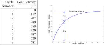
Figure 1.20: Data for Example 1.7.2, simulation of infusion of chemical waste product in a lake.

CHAPTER 1. MATHEMATICAL MODELS OF BIOLOGICAL PROCESSES

Exercises for Section 1.7 Movement toward equilibrium. Exercise 1.7.1 For each of the following systems,

1. Compute W 0 , W u W 2 , W 3 , and W 4 .

2. Find the equilibrium value of W t for the systems.

3. Write a solution equation for the system.

4. Compute Wioo-

5. Compute the half-life, Ti/ 2 = — log 2/ \ogB of the system.

a. W 0 = 0 b. W 0 = 0

W t+1 = 1 + 0.2W* W t+1 = 10 + 0.2W

c. Wo = 0 d. Wo = 0

W t+ i = 100 + 0.2W t W t+ i = 10 + 0.1Wi

e. Wo = 0 f. Wo = 0

W t+1 = 10 + 0.05W W t+1 = 10 + 0.01W t

Exercise 1.7.2 For each of the following systems,

1. Compute W 0 , W u W 2 , W 3 , and W A .

2. Find the equilibrium value of W t for the systems.

3. Write a solution equation for the system.

4. Compute Woo-

a. W 0 = 0 b. Wo = 0

Wi+i = 1-0.2W Wt+i = 10-0.2W

c. Wo = 0 d. W 0 = 0

W+i = 100-0.2W W m = 10-0.1W

e. W 0 = 0 f. Wo = 0

Wt+i = 10-0.05W Wt+i = 10-0.01W

Exercise 1.7.3 For each of the following systems,

a. Compute W 0 , Wi, W 2 , W 3 , and W 4 .

CHAPTER 1. MATHEMATICAL MODELS OF BIOLOGICAL PROCESSES

40

a.

W 0 W t+1

0

i-w t

b.

w 0 w t+1

1

2

i-w t

c.

Wo = 0 W t+1 = 1 + W t

d.

W 0 = 0 W t+1 = 2 + W t

c.

Wo

w +1

0

1 + 2W

f.

Wo

w +1

-1

1 + 2W t

Exercise 1.7.4 Write equations and solve them to describe the amount of salt in the beakers at the beginning of each cycle for the simulation of chemical discharge into a lake of Example 1.7.2.

Exercise 1.7.5 For our model, 1.7.1, of lake pollution, we assume “that upon release from the factory, the chemical quickly mixes throughout the lake so that the chemical concentration in the lake is uniform.” The time scale for ‘quickly’ is relative to the other parts of the model; in this case to the daily flow into and out of the lake. Suppose it takes 10 days for 100 kg of chemical released from the factory to mix uniformly throughout the lake. Write a mathematical model for this case. There are several reasonable models; your task to write one of them.

Exercise 1.7.6 An intravenous infusion of penicillin is initiated into the vascular pool of a patient at the rate of 10 mg penicillin every five minutes. The patients kidneys remove 20 percent of the penicillin in the vascular pool every five minutes.

a. Write a mathematical model of the change during each five minute period of penicillin in the patient.

b. Write a difference equation that describes the amount of penicillin in the patient during the five minute intervals.

c. What is the initial value of penicillin in the patient?

d. What will be the equilibrium amount of penicillin in the patient? (This is important to the nurse and the doctor!)

e. Write a solution to the difference equation.

f. At what time will the penicillin amount in the patient reach 90 percent of the equilibrium value? (The nurse and doctor also care about this. Why?)

g. Suppose the patients kidneys are weak and only remove 10 percent of the penicillin in the vascular pool every 5 minutes. What is the equilibrium amount of penicillin in the patient?

Exercise 1.7.7 The nitrogen partial pressure in a muscle of a scuba diver is initially 0.8 atm. She descends to 30 meters and immediately the N2 partial pressure in her blood is 2.4 atm, and remains at 2.4 atm while she remains at 30 meters. Each minute the N2 partial pressure in her muscle increases by an amount that is proportional to the difference in 2.4 and the partial pressure of nitrogen in her muscle at the beginning of that minute.

a. Write a dynamic equation with initial condition to describe the N2 partial pressure in her muscle.

CHAPTER 1. MATHEMATICAL MODELS OF BIOLOGICAL PROCESSES

41

b. Your dynamic equation should have a proportionality constant. Assume that constant to be 0.067. Write a solution to your dynamic equation.

c. At what time will the N 2 partial pressure be 1.6?

d. What is the half-life of N 2 partial pressure in the muscle, with the value of K — 0.067?

1.8 Solution to the dynamic equation P t+ \ — P t = r P t + b.

The general form of the dynamic equation of the previous section is,

P t+1 -p t = r p t + b, t = 0,1, • • •, P 0 a known value. (1.24)

The constant b represents influence from outside the system, such as flow or immigration into (b > 0) or flow or emigration out of (b < 0) the system. Suppose r 0 and 6^0. We convert

P t+ i-P t = rP t + b

to iteration form

P t+1 = RP t + b, where R = r + 1. (1.25) Next we look for an equilibrium value E satisfying

E = RE + b. (1.26)

(Think, if P t = E then P t+1 = E.) We can solve for E

Now subtract Equation 1.26 from Equation 1.25.

P t+1 = RP t + b E = RE+b

Pt+i-E = R(P t -E). (1.28)

Let D t = P t — E and write

D t+l = RD t .

This is iteration Equation 1.7 with D T instead of P t and the solution is

D t — R l .Do-Remembering that D t = P t — E and E — 6/(1 — R) — —b/r and R = 1 + r we write

P t -E = R t (P 0 – E), Pt = h ~ + {P 0 + £)(! + rf. (1.29) You are asked to show in Exercise 1.8.2 that the solution to

CHAPTER 1. MATHEMATICAL MODELS OF BIOLOGICAL PROCESSES

42

Exercises for Section 1.8, Solution to the dynamic equation, P t+1 — P t = rP t + b.

Exercise 1.8.1 Write a solution equation for the following initial conditions and difference equations or iteration equations. In each case, compute B wo .

Exercise 1.8.2 Equation 1.30

Pt+i -Pt = b

represents a large number of equations

Pi-Po = b P2-P1 = b P3-P2 = b

Pn-l — Pn-2 — b Pn — Pn-l = b

Add these equations to obtain

P n = P 0 + n b

Substitute t for n to obtain

Pt = Po + tb

Exercise 1.8.3 Suppose a quail population would grow at 20% per year without hunting pressure, and 1000 birds per year are harvested. Describe the progress of the population over 5 years if initially there are

a. 5000 birds, b. 6000 birds, and c. 4000 birds. 1.9 Light Decay with Distance.

Example 1.9.1 Some students measured the intensity of light from a 12 volt light bulb with 0.5 amp current at varying distances from the light bulb. The light decreases as the distance from the bulb increases, as shown in Figure 1.21 A.

If the data are transformed as shown in Figure 1.21B then they become very interesting. For each point, (d,I) of Figure 1.21A, the point (l/d 2 ,I) is plotted in Figure 1.21B. Light intensity vs the reciprocal of the square of the distance from the light source is shown. It looks pretty linear.

Explore 1.9.1 a. One data point is omitted from Figure 1.21B. Compute the entry and plot the corresponding point on the graph. Note the factor x 10 -3 on the horizontal scale. The point 2.5 on the horizontal scale is actually 2.5 x 10~ 3 = 0.0025.

CHAPTER 1. MATHEMATICAL MODELS OF BIOLOGICAL PROCESSES

43

A

B

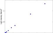
Distance from light source in cm

1/d d = dist from light in cm

Distance cm 20 25 30 40 50 70 100 150 200

Light Intensity

mW/cm 2 0.133 0.086 0.061 0.034 0.024 0.011 0.005 0.002 0.001

Figure 1.21: A. Light intensity vs distance from light source. B. Light intensity vs the reciprocal of the square of the distance from the light source. The light intensity is measured with a Texas Instruments Calculator Based Laboratory (CBL) which is calibrated in milliwatts/cm 2 = mW/cm 2 .

b. Explain why it would be reasonable for some points on the graph to be close to (0,0) in Figure 1.21B.

c. Is (0,0) a possible data point for Figure 1.21B?

It appears that we have found an interesting relation between light intensity and distance from a light source. In the rest of this section we will examine the geometry of light emission and see a fundamental reason suggesting that this relation would be expected, h

In Section 1.3 we saw that sunlight decayed exponentially with depth in the ocean. In Example 1.9.1 we saw that light decreased proportional to the reciprocal of the square of the distance from the light source. These two cases are distinguished by the model of light decrease, and the crux of the problem is the definition of light intensity, and how the geometry of the two cases affects light transmission, and the medium through which the light travels.

Light Intensity. Light intensity from a certain direction is defined to be the number of photons per second crossing a square meter region that is perpendicular to the chosen direction.

The numerical value of light intensity as just defined is generally large – outside our range of experience – and may be divided by a similarly large number to yield a measurement more practical to use. For example, some scientists divide by Avagadro’s number, 6.023 10 23 . A more standard way is to convert photons to energy and photons per second to watts and express light intensity in watts per meter squared.

Light rays emanating from a point source expand radially from the source. Because of the distance between the sun and Earth, sun light strikes the Earth in essentially parallel rays and light intensity remains constant along the light path, except for the interference from substance along the path.

CHAPTER 1. MATHEMATICAL MODELS OF BIOLOGICAL PROCESSES

44

When light is measured ‘close to’ a point source, however, the light rays expand and light intensity decreases as the observer moves away from the source. Consider a cone with vertex V at a point source of light. The number of photons per second traveling outward within the solid is cone constant. As can be seen in Figure 1.22, however, because the areas of surfaces stretching across the cone expand as the distance from the source increases, the density of photons striking the surfaces decreases.

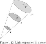
Mathematical Model 1.9.1 Light Expansion: For light emanating uniformly from a point source and traveling in a solid cone, the number of photons per second crossing the surface of a sphere with center at the vertex of the cone is a constant, N, that is, independent of the radius of the sphere.

Because light intensity is ‘number of photons per second per square meter of surface’ we have

N = I d A d (1.31)

where

N is photons per second in a solid cone emanating from a light source

at the vertex of the cone. d is distance from the light source. Id is light intensity at distance d. Ad is the area of the intersection with the cone of

the surface of a sphere of radius d and center at the vertex of the cone.

Illustrated in Figure 1.23 is a cone with vertex V, a sphere with center V and radius d and the portion of the surface of the sphere that lies within the cone. If the vertex angle is a then

CHAPTER 1. MATHEMATICAL MODELS OF BIOLOGICAL PROCESSES 45 Therefore in N = Ij A^

N = I d 2tt(1 – cos a) d 2

or

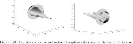
Thus it is not a surprise that in Example 1.9.1, the intensity of light emanating from the 12 volt, 0.5 amp bulb was proportional to the reciprocal of the square of the light intensity.

For light emanating from a point source, the light intensity on the surface of a sphere with center at the point source and radius d is a constant, that is, the light intensity is the same at any two points of the sphere.

Exercise 1.9.1 Shown in Table 1.9.1 is data showing how light intensity from a linear light source decreases as distance from the light increases. Card board was taped on the only window in a room so that a one centimeter wide vertical slit of length 118 cm was left open. For this experiment, we considered 118 cm slit to be an infinitely long line of light. Other lights in the room were cut off. A light meter was pointed horizontally towards the center of the slit, 56 cm above the bottom of the slit, and light intensity was measured as the light meter was moved away from the window.

a. This experiment is easy to replicate. Try and use your own data for the next two parts. Best to have either a clear day or an overcast day; constant sunlight is needed.

b. Light emitted from a point surface is constant on surfaces of spheres with center at the light source. On which surfaces would you expect the intensity of light emitted from a linear source be constant?

c. (You may wish to do the next part before this one.) Explore the data and see whether you can find a relation between light intensity and some aspect of distance.

d. Formulate a model of how light decays with distance from a slit light source and relate your model to your observed relation.

CHAPTER 1. MATHEMATICAL MODELS OF BIOLOGICAL PROCESSES

46

Table for Exercise 1.9.1 Light intensity from a 1 cm strip of light measured at distances perpendicular to the strip.

Distance (cm) 3 4 5 6 7 8 9

Light Intensity mW/cm 2 0.474 0.369 0.295 0.241 0.208 0.180 0.159

Distance (cm) 10 11 12 13 14 15 16

Light Intensity mW/cm 2 0.146 0.132 0.120 0.111 0.100 0.092 0.086

1.10 Data modeling vs mathematical models.

In Example 1.9.1 of light intensity from a 12 volt bulb we modeled data and only subsequently built a mathematical model of light decrease from a point source of light. There are other examples of modeling of data that are interesting but there is very little possibility of building a mathematical model to explain the process. See Also: http: //mathinsight.org/data_modeling_versusjnathematicaLmodeling

Example 1.10.1 Jack A. Wolfe 14 observed that leaves of trees growing in cold climates tend to be incised (have ragged edges) and leaves of trees growing in warm climates tend to have smooth edges (lacking lobes or teeth). He measured the percentages of species that have smooth margins among all species of the flora in many locations in eastern Asia. His data, as read from a graph in U. S. Geological Survey Professional Paper 1106, is presented in Figure 1.10.0.2.

Figure for Example 1.10.0.2 Average temperature C° vs percentage of tree species with smooth edge leaves in 33 forests in eastern Asia. The equation of the line is y — —0.89 + 0.313x.

2 15

0 10 20 30 40 50 60 70 80 90

Percent smooth leaves

The line, temp = 0.89 + 0.313 % smooth is shown in Figure 1.10.0.2 and is close to the data. The line was used by Wolfe to estimate temperatures over the last 65 million years based on observed fossil leaf composition (Exercise 1.10.1). The prospects of writing a mathematical model describing the relationship of smooth edge leaves to temperature are slim, however. ■

Example 1.10.1 On several nights during August and September in Ames, Iowa, some students listened to crickets chirping. They counted the number of chirps in a minute (chirp rate, R) and also recorded the air (ambient) temperature (T) in F° for the night. The data were collected between 9:30 and 10:00 pm each night, and are shown in the table and graph in Figure 1.24.

14 Jack A. Wolfe, A paleobotanical interpretation of tertiary climates in northern hemisphere, American Scientist 66 (1979), 694-703

CHAPTER 1. MATHEMATICAL MODELS OF BIOLOGICAL PROCESSES

47

Ambient Temperature – Fahrenheit

Figure 1.24: A table and graph of the frequency of cricket chirps vs temperature in degrees F°.

These data also appear linear and the line through (65,100) and (75,145)

R – 100 145 – 100

T – 65 75 – 65

R = 4.5T – 192.5 (1.32)

lies close to the data. We can use the line to estimate temperature to be about 69.5 F° if cricket chirp rate is 120 chirps/minute.

This observation was made by Amos Dolbear in 1897, see National Geographic July 2012, 222 (l), P 17ff. –

Both of these examples are examples of data modeling. We fit a line to the data, but there is no underlying explanation of what mechanism is causing the relation.

Exercises for Section 1.10, Data modeling vs mathematical models.

Exercise 1.10.1 Jack Wolfe applied his data (Figure 1.10.0.2) to resolve a dispute about estimates of ambient temperatures during the last 65 million years. Fossil leaves from strata ranging in age back to 65 million years were examined for the percent of smooth-leafed species in each stratum. Under the hypothesis that the relation between percent of smooth-leafed species and temperature in modern species persisted over the last 65 million years, he was able to estimate the past temperatures. Your job is to replicate his work. Although Wolfe collected fossil leaf data from four locations ranging from southern Alaska to Mississippi, we show only his data from the Pacific Northwest, in Table Ex. 1.10.1, read from a graph in Wolfe’s article in American Scientist 1979, 66:694-703.

Use the Percent Smooth data for the fossil leaves at previous times in Table Ex. 1.10.1, and the modern relation, temp = 0.89 + 0.313 % smooth, to draw a graph showing the history of ambient temperature for the land of the Pacific Northwest

a. Over the period from 50 to 40 million years ago.

b. Over the period from 35 to 26 million years ago.

CHAPTER 1. MATHEMATICAL MODELS OF BIOLOGICAL PROCESSES

48

c. Over the period from 26 to 16 million years ago.

d. Over the period from 16 to 6 million years ago.

Table for Exercise 1.10.1 Percentages of smooth-leafed species found in geological strata in the Pacific Northwest.

Exercise 1.10.2 a. Use the graph in Figure 1.24 to estimate the expected temperature if the cricket chirp rate were were 95 chirps per minute? Also use Equation 1.32 to compute the same temperature and compare your results.

b. On the basis of Equation 1.32, what cricket chirp frequencies might be expected for the temperatures 110 °F and 40 °F? Discuss your answers in terms of the data in Figure 1.24 and the interval on which the equation is valid.

c. A television report stated that in order to tell the temperature, count the number of cricket chirps in 13 seconds and add 40. The result will be the temperature in Fahrenheit degrees. Is that consistent with Equation 1.32? (Suggestion: Solve for Temperature °F in terms of Cricket Chirps per Minute.)

Exercise 1.10.3 Some students made a small hole near the bottom of the cylindrical section of a two-liter plastic beverage container, held a finger over the hole and filled the container with water to the top of the cylindrical section, at 15.3 cm. The small hole was uncovered and the students marked the height of the water remaining in the tube, reported here at eighty-second intervals, until the water ran out. They then measured the heights of the marks above the hole. The data gathered and a graph of the data are shown in Figure 1.25.

a. Select a curve and fit an equation for the curve to the data in Figure 1.25.

b. Search your physics book for a mathematical model that explains the data. A fluid dynamicist named Evangelista Torricelli (1608-1649) provided such a model (and also invented the mercury thermometer).

c. The basic idea of Torricelli’s formula is that the potential energy of a thin layer of liquid at the top of the column is converted to kinetic energy of fluid flowing out of the hole.

Let the time index, to, t\, ■ ■ ■ measure minutes and hk be the height of the water at time tk-The layer between hk and hk+i has mass m k and potential energy rrikghk- During the kth

CHAPTER 1. MATHEMATICAL MODELS OF BIOLOGICAL PROCESSES

49

Time sec

Figure 1.25: Height of water draining from a 2-liter beverage container measured at 40 second intervals.

minute an equal mass and volume of water flows out of the hole with velocity, v k , and kinetic energy \m k v\. Equating potential and kinetic energies,

m k gh k = -m k vl, gh k = -vl

Let A cy i inc jer and Ahoie be the cross-sectional areas of the cylinder and hole, respectively.

1. Argue that

-^-cylinder h k -^cylinder /; ; \

v k = —r = —r [h k — hk+i)

Ahole t k+ i — t k ^hole

2. Argue that

hk+i = h k – K\fh~ k (1.33)

where K is a constant.

3. Compare Equation 1.33 with Equation 1.18

1.11 Summary

You have begun one of the most important activities in science, the writing of mathematical models. The best models are sufficiently detailed in their description that dynamic equations describing the progress of the underlying system can be written and lead to solution equations that describe the overall behavior. In our models there was a quantity (Q) that changed with either time or distance (v) and the dynamic equation specified how the change in Q, Q v+ i — Q v , depended on Q or v. The solution equation explicitly expressed the relation of Q to v.

In some cases, such as the case of cricket chirp frequency dependence on ambient temperature in Example 1.10.1, the underlying mechanism is too complex to model it. The observation, however, stimulates considerable thought about why it should be. Presumably the metabolism of the cricket increases with temperature thus causing an increase in chirp frequency, but the phrase, ‘metabolism of the cricket’, masks a large complexity.

We have generally followed certain steps in developing our models. They are useful steps but by no means do they capture the way to model the biological universe. The modeling process is varied and has to be adapted to the questions at hand.

CHAPTER 1. MATHEMATICAL MODELS OF BIOLOGICAL PROCESSES

50

By the methods of this chapter you can solve every first order linear finite difference equation with constant coefficients:

Vo given, y t+1 – y t = r y t + b (1.34)

The solution is

y t = — + (y 0 + -) (r + 1)* if r ^ 0, or y t = y 0 + t b if r = 0.

r r

Exercises for Chapter 1, Mathematical Models of Biological Processes.

Chapter Exercise 1.11.1 Two kilos of a fish poison, rotenone, are mixed into a lake which has a volume of 100 x 20 x 2 = 4000 cubic meters. No water flows into or out of the lake. Fifteen percent of the rotenone decomposes each day.

a. Write a mathematical model that describes the daily change in the amount of rotenone in the lake.

b. Let R 0 , Pi, R 2 , ■ ■ ■ denote the amounts of rotenone in the lake, P t being the amount of poison in the lake at the beginning of the tth day after the rotenone is administered. Write a dynamic equation representative of the mathematical model.

c. What is i? 0 ? Compute Ri from your dynamic equation. Compute R 2 from your dynamic equation.

d. Find a solution equation for your dynamic equation.

Note: Rotenone is extracted from the roots of tropical plants and in addition to its use in killing fish populations is used as a insecticide on such plants as tomatoes, pears, apples, roses, and African violets. Studies in which large amounts (2 to 3 mg/Kg body weight) of rotenone were injected into the jugular veins of laboratory rats produced symptoms of Parkinson’s disease, including the reduction of dopamine producing cells in the brain. (Benoit I. Giasson & Virginia M.-Y. Lee, A new link between pesticides and Parkinson’s disease, Nature Neuroscience 3, 1227 – 1228 (2000)).

Chapter Exercise 1.11.2 Two kilos of a fish poison that does not decompose are mixed into a lake that has a volume of 100 x 20 x 2 = 4000 cubic meters. A stream of clean water flows into the lake at a rate of 1000 cubic meters per day. Assume that it mixes immediately throughout the whole lake. Another stream flows out of the lake at a rate of 1000 cubic meters per day.

a. Write a mathematical model that describes the daily change in the amount of poison in the lake.

b. Let Pq, Pi, P 2 , ■ ■ ■ denote the amounts of poison in the lake, Pt being the amount of poison in the lake at the beginning of the tth day after the poison is administered. Write a dynamic equation representative of the mathematical model.

c. What is Pq! Compute P\ from your dynamic equation. Compute P 2 from your dynamic equation.

d. Find a solution equation for your dynamic equation.

CHAPTER 1. MATHEMATICAL MODELS OF BIOLOGICAL PROCESSES

51

Chapter Exercise 1.11.3 Two kilos of rotenone are mixed into a lake which has a volume of 100 x 20 x 2 = 4000 cubic meters. A stream of clean water flows into the lake at a rate of 1000 cubic meters per day. Assume that it mixes immediately throughout the whole lake. Another stream flows out of the lake at a rate of 1000 cubic meters per day. Fifteen percent of the rotenone decomposes every day.

a. Write a mathematical model that describes the daily change in the amount of rotenone in the lake.

b. Let Rq, Ri, i?2, • • • denote the amounts of rotenone in the lake, R t being the amount of rotenone in the lake at the beginning of the tth day after the poison is administered. Write a dynamic equation representative of the mathematical model.

c. What is R 0 ? Compute Ri from your dynamic equation. Compute R 2 from your dynamic equation.

d. Find a solution equation for your dynamic equation. Chapter Exercise 1.11.4 Consider a chemical reaction

A + B — > AB

in which a chemical, A, combines with a chemical, B, to form the compound, AB. Assume that the amount of B greatly exceeds the amount of A, and that in any second, the amount of AB that is formed is proportional to the amount of A present at the beginning of the second. Write a dynamic equation for this reaction, and write a solution equation to the dynamic equation.

Chapter Exercise 1.11.5 An egg is covered by a hen and is at 37° C. The hen leaves the nest and the egg is exposed to 17° C air. After 20 minutes the egg is at 34° C.

Draw a graph representative of the temperature of the egg t minutes after the hen leaves the

nest.

Mathematical Model. During any short time interval while the egg is uncovered, the decrease in egg temperature is proportional to the difference between the egg temperature and the air temperature.

a. Introduce notation and write a dynamic equation representative of the mathematical model.

b. Write a solution equation for your dynamic equation.

c. Your dynamic equation should have one parameter. Use the data of the problem to estimate the parameter.

Chapter Exercise 1.11.6 The length of an burr oak leaf was measured on successive days in May. The data are shown in Table 1.5. Select an appropriate equation to approximate the data and compute the coefficients of your equation. Do you have a mathematical model of leaf growth?

Chapter Exercise 1.11.7 Atmospheric pressure decreases with increasing altitude. Derive a dynamic equation from the following mathematical model, solve the dynamic equation, and use the data to evaluate the parameters of the solution equation.

CHAPTER 1. MATHEMATICAL MODELS OF BIOLOGICAL PROCESSES

52

Table 1.5: Length of a burr oak leaf.

Day May 7 May 8 May 9 May 10 May 11 Length mm 67 75 85 98 113

Mathematical Model 1.11.1 Mathematical Model of Atmospheric Pressure. Consider a vertical column of air based at sea level divided at intervals of 10 meters and assume that the temperature of the air within the column is constant, say 20°C The pressure at any height is the weight of air in the column above that height divided by the cross sectional area of the column. In a 10-meter section of the column, by the ideal gas law the the mass of air within the section is proportional to the product of the volume of the section and the pressure within the section (which may be considered constant and equal to the pressure at the bottom of the section). The weight of the air above the lower height is the weight of air in the section plus the weight of air above the upper height.

Sea-level atmospheric pressure is 1 atm and the pressure at 18,000 feet is one-half that at sea level (an easy to remember datum from NASA).

Figure for Exercise 1.11.7 Figure for Exercise 1.11.7.

Chapter 2

Functions as Descriptions of Biological Patterns.

Where are we going?

Relations between quantities are so central to science and mathematics that the concept has been carefully defined and is named function. You will see how tables of data, graphs, and equations are unified into a single concept, function. This chapter will present examples of some unusual relations between quantities that suggest the usefulness of the general concept, and it will introduce three definitions of function with increasing levels of precision.

Electrocardiograms are examples of relations between voltage and time that are functions. Equations to describe the relation are difficult to find, and once found, are not informative. It is better to think of each trace as simply a function.

Many biological relations may be described by equations — linear, quadratic, hyperbolic, exponential, and logarithmic. These together with the trigonometric equations cover most of the commonly encountered equations. Scientific calculators readily compute these values that in the past were laboriously computed by hand and recorded in lengthy tables. There are some relations between measured quantities that are not so easily described by equations, and in this chapter we see how we can extend the use of equations to describe relations to a general concept referred to as a function. Formal definitions of function and ways of combining functions are presented.

2.1 Environmental Sex Determination in Turtles

It is a well known, but little understood fact that the sex of some reptiles depends on the environment in which the egg is incubated (temperature is important), and is not purely a genetic

CHAPTER 2. DESCRIPTIONS OF BIOLOGICAL PATTERNS

54

determination. A graph of some data on a species of fresh water turtles appears in Figure 2.1 .

Explore 2.1.1 Examine the graph for Chrysemys picta and write a brief verbal description of the dependence of the percentage of females on incubation temperature for a clutch of Chrysemys picta eggs.

26 28

Incubation temperature

Figure 2.1: Percent female hatchlings from incubation of Chrysemys picta eggs at various temperatures.

Your experience probably does not include a single analytic formula that describes the dependence of the percentage of females on incubation temperature for a clutch of turtle eggs. It is easiest to use a piecewise definition; use one formula for a range of temperatures and other formulas for other ranges of temperatures. Your verbal description in the case of Chrysemys picta could say that if the temperature is less than 28 °C, the percent of female is zero, and if the temperature is greater than or equal to 29 °C, the percent of female is 100. One could describe what happens between 28 °C and 29 °C, but the accuracy of the data probably does not warrant such a refinement. This piecewise procedure of describing data occurs often enough to have a special notation.

f 0 if Temp < 28 °C

Percent of hatchlings that are female = < Uncertain if 28 °C < Temp < 29 °C (2-1)

( 100 if 29 °C < Temp

The designation Uncertain for 28 °C < Temp < 29 °C is a bit unsatisfactory but we hope the example sufficiently illustrates piecewise definition of dependence.

Exercises for Section 2.1 Environmental Sex Determination in Turtles.

x This data was collected by Ralph Ackerman from a number of publications, most of which are referenced in, Fredric J. Janzen and Gary L. Paukstis, Environmental sex determination in reptiles: Ecology, evolution, and experimental design, The Quarterly Review of Biology 66 (1991) 149-179.

CHAPTER 2. DESCRIPTIONS OF BIOLOGICAL PATTERNS

55

Exercise 2.1.1 Data on the temperature determination of sex for the snapping turtle, Chelydra serpentina appears in Figure Ex. 2.1.1.

a. Write a verbal description of the dependence of the percentage of females on incubation temperature for a clutch of Chelydra serpentina eggs.

b. Write formulas similar to Formulas 2.1 to describe the dependence of the percentage of females on incubation temperature for a clutch of Chelydra serpentina eggs.

Figure for Exercise 2.1.1 Percent females from clutches of Chelydra serpentina (snapping turtle)

eggs incubated at various temperatures.

Temperature centigrade

2.2 Functions and Simple Graphs.

A large part of science may be described as the study of the dependence of one measured quantity on another measured quantity. The word function is used in this context in a special way. In previous examples, the word function may have been used as follows:

• The density of V. natriegens is a function of time.

• Light intensity is a function of depth below the surface in an ocean.

• Light intensity is a function of distance from the light source.

• The frequency of cricket chirps is a function of the ambient temperature.

• The percentage of females turtles from a clutch of eggs is a function of the incubation temperature.

2.2.1 Three definitions of “Function”.

Because of its prevalence and importance in science and mathematics, the word function has been defined several ways over the past three hundred years, and now is usually given a very precise formal meaning. More intuitive meanings are also helpful and we give three definitions of function, all of which will be useful to us.

The word variable means a symbol that represents any member of a given set, most often a set of numbers, and usually denotes a value of a measured quantity. Thus density of V. natriegens,

CHAPTER 2. DESCRIPTIONS OF BIOLOGICAL PATTERNS

56

time, percentage of females, incubation temperature, light intensity, depth and distance are all variables.

The terms dependent variable and independent variable are useful in the description of an experiment and the resulting functional relationship. The density of V. natriegens (dependent variable) is a function of time (independent variable). The percentage of females turtles from a clutch of eggs (dependent variable) is a function of the incubation temperature (independent variable).

Using the notion of variable, a function may be defined:

Definition 2.2.1 Function I Given two variables, x and y, a function is a rule that assigns to each value of x a unique value ofy.

In this context, x is the independent variable, and y is the dependent variable. In some cases there is an equation that nicely describes the ‘rule’; in the percentage of females in a clutch of turtle eggs examples of the preceding section, there was not a simple equation that described the rule, but the rule met the definition of function, nevertheless.

The use of the words dependent and independent in describing variables may change with the context of the experiment and resulting function. For example, the data on the incubation of turtles implicitly assumed that the temperature was held constant during incubation. For turtles in the wild, however, temperature is not held constant and one might measure the temperature of a clutch of eggs as a function of time. Then, temperature becomes the dependent variable and time is the independent variable.

In Definition 2.2.1, the word ‘variable’ is a bit vague, and ‘a function is a rule’ leaves a question as to ‘What is a rule?’. A ‘set of objects’ or, equivalently, a ‘collection of objects’, is considered to be easier to understand than ‘variable’ and has broader concurrence as to its meaning. Your previous experience with the word function may have been that

Definition 2.2.2 Function II A function is a rule that assigns to each number in a set called the domain a unique number in a set called the range of the function.

Definition 2.2.2 is similar to Definition 2.2.1, except that ‘a number in a set called the domain’ has given meaning to independent variable and ‘a unique number in a set called the range’ has given meaning to dependent variable.

The word ‘rule’ is at the core of both definitions 2.2.1 Function I. and 2.2.2 Function II. and is still a bit vague. The definition of function currently considered to be the most concise is:

Definition 2.2.3 Function III A function is a collection of ordered number pairs no two of which have the same first number.

A little reflection will reveal that ‘a table of data’ is the motivation for Definition 2.2.3. A data point is actually a number pair. Consider the tables of data shown in Table 2.1 from V. natriegens growth and human population records. (16,0.036) is a data point. (64,0.169) is a data point. (1950,2.52) and ( 1980,4.45) are data points. These are basic bits of information for the functions. On the other hand, examine the data for cricket chirps in the same table, from Chapter I. That also is a collection of ordered pairs, but the collection does not satisfy Definition 2.2.3. There are two ordered pairs in the table with the same first term – (66,102) and (66,103). Therefore the collection contains important information about the dependence of chirp frequency on temperature, although the collection does not constitute a function.

In a function that is a collection of ordered number pairs, the first number of a number pair is always a value of the independent variable and a member of the domain and the second number is

CHAPTER 2. DESCRIPTIONS OF BIOLOGICAL PATTERNS

Table 2.1: Examples of tables of data

57

Cricket Chirps

always a value of the dependent variable and a member of the range. Almost always in recording the results of an experiment, the numbers in the domain are listed in the column on the left and the numbers in the range are listed in the column on the right. Formally,

Definition 2.2.4 Domain and Range For Definition 2.2.3 of function, the domain is defined as the set of all numbers that occur as the first number in an ordered pair of the function and the range of the function is the set of all numbers that occur as a second number in an ordered pair of the function.

Example 2.2.1 Data for the percentage of U.S. population in 1955 that had antibodies to the polio virus as a function of age is shown in Table 2.2.1.1. The data show an interesting fact that a high percentage of the population in 1955 had been infected with polio. A much smaller percentage were crippled or killed by the disease.

Although Table 2.2.1.1 is a function, it is only an approximation to a perhaps real underlying function. The order pair, (17.5, 72), signals that 72 percent of the people of age 17.5 years had antibodies to the polio virus. More accurately, (17.5,72) signals that of a sample of people who had ages in the interval from age 15 to less than 20, the percentage who tested positive to antibodies to the polio virus was greater than or equal to 71.5 and less than 72.5.

Table 2.2.1.1 is a useful representation of an enormous table of data that lists for a certain instance of time during 1955, for each U.S. citizen, their age (measured perhaps in hours (minutes?, seconds?)), and whether they had HIV antibodies, ‘y es ‘ or ‘ no >’ This table would not be a function, but for each age, the percent of people of that age who were HIV positive would be a number and those age-percent pairs would form a function. The domain of that function would be the finite set of ages in the U.S. population.

Table for Example 2.2.1.1 Data for percentage of the U.S. population in 1955 at various ages that had antibodies to the polio virus. Data read from Anderson and May, Vaccination and herd immunity to infectious diseases, Nature 318 1985, pp 323-9, Figure 2f.

CHAPTER 2. DESCRIPTIONS OF BIOLOGICAL PATTERNS

58

Age 0.8 1.5 2.5 3.5 4.5 5.5 6.5 7.5 8.5 9.5 12.5 17.5 22.5 27.5 % 3 6 13 19 27 35 40 43 46 49 64 72 78 87

Remember that only a very few data ‘points’ were listed from the large number of possible points in each of the experiments we considered. There is a larger function in the background of each experiment.

Because many biological quantities change with time, the domain of a function of interest is often an interval of time. In some cases a biological reaction depends on temperature (percentage of females in a clutch of turtle eggs for example) so that the domain of a function may be an interval of temperatures. In cases of spatial distribution of a disease or light intensity below the surface of a lake, the domain may be an interval of distances.

It is implicit in the bacteria growth data that at any specific time, there is only one value of the bacterial density 2 associated with that time. It may be incorrectly or inaccurately read, but a fundamental assumption is that there is only one correct density for that specific time. The condition that no two of the ordered number pairs have the same first term is a way of saying that each number in the domain has a unique number in the range associated with it.

All three of the definitions of function are helpful, as are brief verbal descriptions, and we will rely on all of them. Our basic definition, however, is the ordered pair definition, Definition 2.2.3.

2.2.2 Simple graphs.

Coordinate geometry associates ordered number pairs with points of the plane so that by Definition 2.2.3 a function is automatically identified with a point set in the plane called a simple graph:

Definition 2.2.5 Simple Graph A simple graph is a point set, G, in the plane such that no vertical line contains two points ofG.

The domain of G is the set of x-coordinates of points of G and the range of G is the set of all y-coordinates of points of G.

Note: For use in this book, every set contains at least one element.

The domain of a simple graph G is sometimes called the x-projection of G, meaning the vertical projection of G onto the x-axis and the range of G is sometimes called the y-projection of G meaning the horizontal projection of G onto the y-axis.

A review of the graphs of incubation temperature – percentage of females turtles in Figure 2.1 and Exercise Fig. 2.1.1 will show that in each graph at least one vertical line contains two points of the graph. Neither of these graphs is a simple graph, but the graphs convey useful information.

A circle is not a simple graph. As shown in Figure 2.2A there is a vertical line that contains two points of it. There are a lot of such vertical lines. The circle does contain a simple graph, and

CHAPTER 2. DESCRIPTIONS OF BIOLOGICAL PATTERNS

59

contains one that is ‘as large as possible’. The upper semicircle shown in Figure 2.2B is a simple graph. The points (-1,0) and (1,0) are filled to show that they belong to it. It is impossible to add any other points of the circle to this simple graph and still have a simple graph — thus it is ‘as large as possible’. An equation of the upper semicircle is

y = y/l — x 2 , — 1 < x < 1

The domain of this simple graph is [-1,1], and the range is [0,1]. Obviously the lower semicircle is a maximal simple graph also, and it has the equation

y = —yl — x 2 , — 1 < x < 1

The domain is again [-1,1], and the range is [-1,0].

Figure 2.2: A. A circle; a vertical line contains two point of the circle so that it is not a simple graph. B. A subset of the circle that is a simple graph. C. Another subset of the circle that is a simple graph. The simple graphs in (b) and (c) are maximal in the sense that any point from the circle added to the graphs would create a set that is not a simple graph — the vertical line containing that point would also contain a point from the original simple graph.

There is yet a third simple graph contained in the circle, shown in Figure 2.2C, and it is ‘as large as possible’. An equation for that simple graph is

V

VT^ 2 if -1 < x < 0 -yT^x 2 if 0 < x < 1

The domain is [-1,1] and range is [-1,1] Because of the intuitive advantage of geometry, it is often useful to use simple graphs instead of equations or tables to describe functions, but again, we will use any of these as needed.

Exercises for Section 2.2 Functions and Simple Graphs.

Exercise 2.2.1 Which of the tables shown in Table Ex. 2.2.1 reported as data describing the growth of V. natriegens are functions?

Table for Exercise 2.2.1 Hypothetical data for V. natriegens growing in Nutrient Broth.

Exercise 2.2.2 For the following experiments, determine the independent variable and the dependent variable, and draw a simple graph or give a brief verbal description (your best guess) of the function relating the two.

a. A rabbit population size is a function of the number of coyotes in the region.

b. An agronomist, interested in the most economical rate of nitrogen application to corn, measures the corn yield in test plots using eight different levels of nitrogen application.

c. An enzyme, E, catalyzes a reaction converting a substrate, S, to a product P according to

E + S^ES^E + P

Assume enzyme concentration, [E], is fixed. A scientist measures the rate at which the product P accumulates at different concentrations, [S], of substrate.

d. A scientist titrates a 0.1 M solution of HC1 into 5 ml of an unknown basic solution containing litmus (litmus causes the color of the solution to change as the pH changes).

Exercise 2.2.3 A table for bacterial density for growth of V. natriegens is repeated in Exercise Table 2.2.3. There are two functions that relate population density to time in this table, one that relates population density to time and another that relates population to time index.

a. Identify an ordered pair that belongs to both functions.

b. One of the functions is implicitly only a partial list of the order pairs that belong to it. You may be of the opinion that both functions have that property, but some people may think one is more obviously only a sample of the data. Which one?

c. What is the domain of the other function?

CHAPTER 2. DESCRIPTIONS OF BIOLOGICAL PATTERNS 61 Table for Exercise 2.2.3 Data for V. natriegens growing in pH 6.25 nutrient broth.

Exercise 2.2.4 Refer to the graphs in Figure Ex. 2.2.4.

1. Which of the graphs are simple graphs?

2. For those that are not simple graphs,

(a) Draw, using only the points of the graph, a simple graph that is ‘as large as possible’, meaning that no other points can be added and still have a simple graph.

(b) Draw a second such simple graph.

(c) Identify the domains and ranges of the two simple graphs you have drawn.

(d) How many such simple graphs may be drawn?

Figure for Exercise 2.2.4 Graphs for Exercise 2.2.4. Some are simple graphs; some are not simple graphs.

Exercise 2.2.5 Make a table showing the ordered pairs of a simple graph contained in the graph in Figure Ex. 2.2.5 and that has domain

{-1.5, -1.0, -0.5,0.0,0.5,1.0,1.5}

CHAPTER 2. DESCRIPTIONS OF BIOLOGICAL PATTERNS

62

How many such simple graphs are contained in the graph of Figure Ex. 2.2.5 and that have this domain?

Figure for Exercise 2.2.5 Graph for Exercise 2.2.5.

-1 -0.5 0 0.5 1

Exercise 2.2.6 a. Does every subset of the plane contain a simple graph?

b. Does every subset of the plane contain two simple graphs?

c. Is there a subset of the plane that contains two and only two simple graphs?

d. Is there a line in the plane that is not the graph of a function?

e. Is there a function whose graph is a circle?

f. Is there a simple graph in the plane whose domain is the interval [0,1] (including 0 and 1) and whose range is the interval [0,3]?

g. Is there a simple graph in the plane whose domain is [0,1] and whose range is the y-axis?

Exercise 2.2.7 A bit of a difficult exercise. For any location, A on Earth, let Annual Daytime at A, AD(A), be the sum of the lengths of time between sunrise and sunset at A for all of the days of the year. Find a reasonable formula for AD(X). You may guess or find data to suggest a reasonable formula, but we found proof of the validity of our formula a bit arduous. As often happens in mathematics, instead of solving the actual problem posed, we found it best to solve a ‘nearby’ problem that was more tractable. The 365.24… days in a year is a distraction, the elliptical orbit of Earth is a downright hinderance, and the wobble of Earth on its axis can be overlooked. Specifically, we find it helpful to assume that there are precisely 366 days in the year (after all this was true about 7 or 8 million years ago), the Earth’s orbit about the sun is a circle, the Earth’s axis makes a constant angle with the plane of the orbit, and that the rays from the sun to Earth are parallel. We hope you enjoy the question.

2.2.3 Functions in other settings.

There are extensions of the function concept to settings where the ordered pairs are not ordered number pairs. A prime example of this is the genetic code shown in Figure 2.3. The relation is a true function (no two ordered pairs have the same first term), and during the translation of proteins, the ribosome and the transfer RNA’s use this function reliably.

CHAPTER 2. DESCRIPTIONS

OF BIOLOGICAL PATTERNS

63

Figure 2.3: The genetic code (for human nuclear RNA). Sets of three nucleotides in RNA (codons) are translated into amino acids in the course of proteins synthesis. CAA codes for Gin (glutamine). *AUG codes for Met (methionine) and is also the START codon.

Explore 2.2.1 List three ordered pairs of the genetic code. What is the domain of the genetic code? What is the range of the genetic code? ■

The ordered pair concept is retained in the preceding example; the only change has been in the types of objects that are in the domain and range. When the objects get too far afield from simple numbers, the word transformation is sometimes used in place of function. The genetic code is a transformation of the codons into amino acids and start and stop signals.

Another commonly encountered extension of the kinds of objects in the domain of a function occurs when one physical or biological quantity is dependent on two others. For example, the widely known Charles’ Law in Chemistry can be stated as

„ nRT

where P = pressure in atmospheres, n = number of molecular weights of the gas, R = 0.0820 Atmospheres/degree Kelvin-mol = 8.3 /degree Kelvin-mol (the gas constant), T = temperature in kelvins, and V = volume in liters. For a fixed sample of gas, the pressure is dependent on two quantities, temperature and volume. The domain is the set of all feasible temperature-volume pairs, the range is the set of all feasible pressures. The function in this case is said to be a function of two variables. The ordered pairs in the function are of the form

((x, y),z) , or ((temperature, volume), pressure)

There may also be multivalued transformations. For example, doctors prescribe antibiotics. For each bacterial infection, there may be more than one antibiotic effective against that

CHAPTER 2. DESCRIPTIONS OF BIOLOGICAL PATTERNS

64

bacterium; there may be a list of such antibiotics. The domain would be a set of bacteria, and the range would be a set of lists of antibiotics.

Exercises for Section 2.2.3 Functions in other settings. Exercise 2.2.8 Describe the domain and range for each of the following transformations.

a. Bird identification guide book.

b. A judge sentences defendants to jail terms.

c. The time between sunrise and sunset.

d. Antibiotic side effects.

2.3 Function notation.

It is common to let a letter denote a set of ordered pairs that is a function.

If F denotes a function, then for any ordered pair, (x, y) in F, y is denoted by F(x).

Thus the ordered pair (x, F(x)) is an ordered pair of F. The notation makes it very easy to describe a function by an equation. Instead of

‘Let F be the collection of ordered number pairs to which an ordered pair (x, y) belongs if and only if a; is a number and y = x 2 + x.’

one may write

‘Let F be the function such that for all numbers x, F(x) = x 2 + x.’

Operationally, you will find that often you can simply replace y in an equation by F(x) and define a function. Furthermore, because you are used to using y in an equation, you can often replace F(x) in the definition of a function by y and use the resulting equation which is more familiar.

The following expressions all may be used in the definition of a function.

Observe that some conditions, i ^ 0 and x > 0 and x > 0, are included for some of the expressions. Those conditions describe the domain of the function. For example, the domain of the function / defined by F(x) = log 10 x is the set of positive numbers.

CHAPTER 2. DESCRIPTIONS OF BIOLOGICAL PATTERNS

65

You may also see something like F(x) = VTTx

F(x) = VT

F(x) = log

10

[X

x)

The intention is that the domain is the set of all values of x for which the expressions can be computed even though no restrictions are written. Often the restrictions are based on these rules:

1. Avoid dividing by zero.

2. Avoid computing the square root of negative numbers.

3. Avoid computing the logarithm of 0 and negative numbers.

Assuming we use only real numbers and not complex numbers, complete descriptions of the previous functions would be

/(*) F{x)

y/1 + X , X > — 1

-1 < X < 1

F(x) F(x)

l-x l+x

x^-1

log 10 (x 2 — x) , x < 0 or 1 < x

Use of parentheses. The use of parentheses in the function notation is special to functions and does not mean multiplication. The symbol inside the parentheses is always the independent variable, a member of the domain, and F(x) is a value of the dependent variable, a member of the range. It is particularly tricky in that we will often need to use the symbol F(x + h), and students confuse this with a multiplication and replace it with F(x) + F(h). Seldom is this correct.

Example 2.3.1 For the function, R, defined by

R(x) = x +

x

x^O

R(l + 3) = R(4) = 4 +

R(l) R(3)

3 +

i + Y = 2.o

4.25

and

3.3333′

In this case

R(l) + R(3) = 2 + 3.3333— = 5.3333—^ 4.25 = i?(4)

R(1 + 3)^R(1) + R(3)

CHAPTER 2. DESCRIPTIONS OF BIOLOGICAL PATTERNS

66

Exercises for Section 2.3 Function Notation.

Exercise 2.3.1 Let F be the collection of ordered number pairs to which an ordered pair (x,y) belongs if and only if x is a number and y = x 2 + x.

a. Which of the ordered number pairs belong to F? (0,1), (0,0), (1,1), (1,3), (1,-1), (-1,1), (-1,0), (-1,-1).

b. Is there any uncertainty as to the members of F?

c. What is the domain of F?

d. What is the range of F?

Exercise 2.3.2 For the function, F, defined by F(x) = x 2 ,

1. Compute F(l + 2), and F(l) + F(2). Is F(l + 2) = F(l) + F(2)?

2. Compute F(3 + 5), and F(3) + F(5). Is F(3 + 5) = F(3) + F(5)?

3. Compute F(0 + 4), and F(0) + F(4). Is F(0 + 4) = F(0) + F(4)?

Exercise 2.3.3 Find a function, L, defined for all numbers (domain is all numbers) such that for all numbers a and b, L(a + b) = L(a) + L(b). Is there another such function?

Exercise 2.3.4 Find a function, M, defined for all numbers (domain is all numbers) such that for all numbers a and b, M(a + b) = M(a) x M(b). Is there another such function?

Exercise 2.3.5 For the function, F(x) = x 2 + x, compute the following

( a) m^m (b) f(3+2)-f(3)

/ X F(b)-F(a) /,n F(a+h)-F(a)

\ / b—a \ ‘ h

Exercise 2.3.6 Repeat steps (a) – (d) of Exercise 2.3.5 for the functions

(i) F{x) = 3x (ii) F(x) = x 3

(iii) F(x) = 2 X (iv) F(x) = sin a;

Exercise 2.3.7 a. In Figure 2.3.7A is the graph of y A = x 2 for —2 < x < 2. Write equations that define five different maximal simple subgraphs.

b. In Figure 2.3.7B is the graph of \x\ + \y\ = 1 for — 1 < x < 1. Write equations that define five different maximal simple subgraphs.

CHAPTER 2. DESCRIPTIONS OF BIOLOGICAL PATTERNS

67

Exercise 2.3.8 What are the implied domains of the functions

F(x) = F(x) = g£

F(x) = ^4^x2 F(x) = log 10 (x 2 )

2.4 Polynomial functions.

Data from experiments (and their related functions) are often described as being linear, parabolic, hyperbolic, polynomial, harmonic (sines and cosines), exponential, or logarithmic either because their graphs have some resemblance to the corresponding geometric object or because equations describing their related functions use the corresponding expressions. In this section we extend linear and quadratic equations to more general polynomial functions.

Definition 2.4.1 Polynomial For n a positive integer or zero, a polynomial of degree n is a function, P defined by an equation of the form

P(x) = a 0 + ai x + a 2 x 2 + a 3 x 3 + ■ ■ ■ + a n x n

where a 0 , ai, a 2 , a 3 , • • a n are numbers, independent of x, called the coefficients of p ; and ifn>0a n ^0.

Functions of the form

P(x) = C where C is a number

are said to be constant functions and also polynomials of degree zero. Functions defined by equations

P(x)=a + bx and P(x) = a + bx + cx 2

are linear and quadratic polynomials, respectively, and are polynomials of degree one and degree two. The equation

P(x) = 3 + 5a; + 2x 2 + (-4):r 3

is a polynomial of degree 3 with coefficients 3, 5, 2, and -4 and is said to be a cubic polynomial. Polynomials are important for four reasons:

1. Polynomials can be computed using only the arithmetic operations of addition, subtraction, and multiplication.

2. Most functions used in science have polynomials “close” to them over finite intervals. See Figure 2.4, Example 2.5.2, and Exercise 2.5.3.

3. The sum of two polynomials is a polynomial, the product of two polynomials is a polynomial, and the composition of two polynomials is a polynomial.

4. Polynomials are ‘linear’ in their coefficients, a fact which makes them suitable for least squares ‘fit’ to data.

CHAPTER 2. DESCRIPTIONS OF BIOLOGICAL PATTERNS

68

Reason 1 is obvious, but even the meaning of Reason 2 is opaque. An illustration of Reason 2 follows, and we return to the question in Chapter 12. Sum, product, and composition of two functions are described in Section 2.6. Reason 4 is illustrated in Example 2.4.1.