
2.7: The Precise Definition of a Limit
- Page ID
- 20579
\( \newcommand{\vecs}[1]{\overset { \scriptstyle \rightharpoonup} {\mathbf{#1}} } \)
\( \newcommand{\vecd}[1]{\overset{-\!-\!\rightharpoonup}{\vphantom{a}\smash {#1}}} \)
\( \newcommand{\dsum}{\displaystyle\sum\limits} \)
\( \newcommand{\dint}{\displaystyle\int\limits} \)
\( \newcommand{\dlim}{\displaystyle\lim\limits} \)
\( \newcommand{\id}{\mathrm{id}}\) \( \newcommand{\Span}{\mathrm{span}}\)
( \newcommand{\kernel}{\mathrm{null}\,}\) \( \newcommand{\range}{\mathrm{range}\,}\)
\( \newcommand{\RealPart}{\mathrm{Re}}\) \( \newcommand{\ImaginaryPart}{\mathrm{Im}}\)
\( \newcommand{\Argument}{\mathrm{Arg}}\) \( \newcommand{\norm}[1]{\| #1 \|}\)
\( \newcommand{\inner}[2]{\langle #1, #2 \rangle}\)
\( \newcommand{\Span}{\mathrm{span}}\)
\( \newcommand{\id}{\mathrm{id}}\)
\( \newcommand{\Span}{\mathrm{span}}\)
\( \newcommand{\kernel}{\mathrm{null}\,}\)
\( \newcommand{\range}{\mathrm{range}\,}\)
\( \newcommand{\RealPart}{\mathrm{Re}}\)
\( \newcommand{\ImaginaryPart}{\mathrm{Im}}\)
\( \newcommand{\Argument}{\mathrm{Arg}}\)
\( \newcommand{\norm}[1]{\| #1 \|}\)
\( \newcommand{\inner}[2]{\langle #1, #2 \rangle}\)
\( \newcommand{\Span}{\mathrm{span}}\) \( \newcommand{\AA}{\unicode[.8,0]{x212B}}\)
\( \newcommand{\vectorA}[1]{\vec{#1}} % arrow\)
\( \newcommand{\vectorAt}[1]{\vec{\text{#1}}} % arrow\)
\( \newcommand{\vectorB}[1]{\overset { \scriptstyle \rightharpoonup} {\mathbf{#1}} } \)
\( \newcommand{\vectorC}[1]{\textbf{#1}} \)
\( \newcommand{\vectorD}[1]{\overrightarrow{#1}} \)
\( \newcommand{\vectorDt}[1]{\overrightarrow{\text{#1}}} \)
\( \newcommand{\vectE}[1]{\overset{-\!-\!\rightharpoonup}{\vphantom{a}\smash{\mathbf {#1}}}} \)
\( \newcommand{\vecs}[1]{\overset { \scriptstyle \rightharpoonup} {\mathbf{#1}} } \)
\(\newcommand{\longvect}{\overrightarrow}\)
\( \newcommand{\vecd}[1]{\overset{-\!-\!\rightharpoonup}{\vphantom{a}\smash {#1}}} \)
\(\newcommand{\avec}{\mathbf a}\) \(\newcommand{\bvec}{\mathbf b}\) \(\newcommand{\cvec}{\mathbf c}\) \(\newcommand{\dvec}{\mathbf d}\) \(\newcommand{\dtil}{\widetilde{\mathbf d}}\) \(\newcommand{\evec}{\mathbf e}\) \(\newcommand{\fvec}{\mathbf f}\) \(\newcommand{\nvec}{\mathbf n}\) \(\newcommand{\pvec}{\mathbf p}\) \(\newcommand{\qvec}{\mathbf q}\) \(\newcommand{\svec}{\mathbf s}\) \(\newcommand{\tvec}{\mathbf t}\) \(\newcommand{\uvec}{\mathbf u}\) \(\newcommand{\vvec}{\mathbf v}\) \(\newcommand{\wvec}{\mathbf w}\) \(\newcommand{\xvec}{\mathbf x}\) \(\newcommand{\yvec}{\mathbf y}\) \(\newcommand{\zvec}{\mathbf z}\) \(\newcommand{\rvec}{\mathbf r}\) \(\newcommand{\mvec}{\mathbf m}\) \(\newcommand{\zerovec}{\mathbf 0}\) \(\newcommand{\onevec}{\mathbf 1}\) \(\newcommand{\real}{\mathbb R}\) \(\newcommand{\twovec}[2]{\left[\begin{array}{r}#1 \\ #2 \end{array}\right]}\) \(\newcommand{\ctwovec}[2]{\left[\begin{array}{c}#1 \\ #2 \end{array}\right]}\) \(\newcommand{\threevec}[3]{\left[\begin{array}{r}#1 \\ #2 \\ #3 \end{array}\right]}\) \(\newcommand{\cthreevec}[3]{\left[\begin{array}{c}#1 \\ #2 \\ #3 \end{array}\right]}\) \(\newcommand{\fourvec}[4]{\left[\begin{array}{r}#1 \\ #2 \\ #3 \\ #4 \end{array}\right]}\) \(\newcommand{\cfourvec}[4]{\left[\begin{array}{c}#1 \\ #2 \\ #3 \\ #4 \end{array}\right]}\) \(\newcommand{\fivevec}[5]{\left[\begin{array}{r}#1 \\ #2 \\ #3 \\ #4 \\ #5 \\ \end{array}\right]}\) \(\newcommand{\cfivevec}[5]{\left[\begin{array}{c}#1 \\ #2 \\ #3 \\ #4 \\ #5 \\ \end{array}\right]}\) \(\newcommand{\mattwo}[4]{\left[\begin{array}{rr}#1 \amp #2 \\ #3 \amp #4 \\ \end{array}\right]}\) \(\newcommand{\laspan}[1]{\text{Span}\{#1\}}\) \(\newcommand{\bcal}{\cal B}\) \(\newcommand{\ccal}{\cal C}\) \(\newcommand{\scal}{\cal S}\) \(\newcommand{\wcal}{\cal W}\) \(\newcommand{\ecal}{\cal E}\) \(\newcommand{\coords}[2]{\left\{#1\right\}_{#2}}\) \(\newcommand{\gray}[1]{\color{gray}{#1}}\) \(\newcommand{\lgray}[1]{\color{lightgray}{#1}}\) \(\newcommand{\rank}{\operatorname{rank}}\) \(\newcommand{\row}{\text{Row}}\) \(\newcommand{\col}{\text{Col}}\) \(\renewcommand{\row}{\text{Row}}\) \(\newcommand{\nul}{\text{Nul}}\) \(\newcommand{\var}{\text{Var}}\) \(\newcommand{\corr}{\text{corr}}\) \(\newcommand{\len}[1]{\left|#1\right|}\) \(\newcommand{\bbar}{\overline{\bvec}}\) \(\newcommand{\bhat}{\widehat{\bvec}}\) \(\newcommand{\bperp}{\bvec^\perp}\) \(\newcommand{\xhat}{\widehat{\xvec}}\) \(\newcommand{\vhat}{\widehat{\vvec}}\) \(\newcommand{\uhat}{\widehat{\uvec}}\) \(\newcommand{\what}{\widehat{\wvec}}\) \(\newcommand{\Sighat}{\widehat{\Sigma}}\) \(\newcommand{\lt}{<}\) \(\newcommand{\gt}{>}\) \(\newcommand{\amp}{&}\) \(\definecolor{fillinmathshade}{gray}{0.9}\)By now you have progressed from the very informal definition of a limit in the introduction of this chapter to the intuitive understanding of a limit. At this point, you should have a very strong intuitive sense of what the limit of a function means and how you can find it. In this section, we convert this intuitive idea of a limit into a formal definition using precise mathematical language. The formal definition of a limit is quite possibly one of the most challenging definitions you will encounter early in your study of calculus; however, it is well worth any effort you make to reconcile it with your intuitive notion of a limit. Understanding this definition is the key that opens the door to a better understanding of calculus.
Quantifying Closeness
Before stating the formal definition of a limit, we must introduce a few preliminary ideas. Recall that the distance between two points a and b on a number line is given by |\(a−b\)|.
- The statement \(|f(x)−L|<ε\) may be interpreted as: The distance between \(f(x)\) and L is less than \(ε\).
- The statement \(0<|x−a|<δ\) may be interpreted as: \(x≠a\) and the distance between \(x\) and \(a\) is less than \(δ\).
It is also important to look at the following equivalences for absolute value:
- The statement \(|f(x)−L|<ε\) is equivalent to the statement \(L−ε<f(x)<L+ε\).
- The statement \(0<|x−a|<δ\) is equivalent to the statement \(a−δ<x<a+δ\) and \(x≠a\).
With these clarifications, we can state the formal epsilon-delta definition of the limit.
Definition: The Epsilon-Delta Definition of the Limit
Let \(f(x)\) be defined for all \(x≠a\) over an open interval containing a. Let L be a real number. Then
\[\displaystyle \lim_{x→a}f(x)=L\]
if, for every \(ε>0\), there exists a \(δ>0\), such that if \(0<|x−a|<δ\), then \(|f(x)−L|<ε\).
This definition may seem rather complex from a mathematical point of view, but it becomes easier to understand if we break it down phrase by phrase. The statement itself involves something called a universal quantifier (for every \(ε>0\)), an existential quantifier (there exists a \(δ>0\)), and, last, a conditional statement (if \(0<|x−a|<δ\), then \(|f(x)−L|<ε)\). Let’s take a look at Table, which breaks down the definition and translates each part.
| Definition | Translation |
|---|---|
| 1. For every \(ε>0\), | 1. For every positive distance \(ε\) from \(L\) , |
| 2. there exists a \(δ>0\), | 2. There is a positive distance \(δ\) from \(a\) , |
| 3. such that | 3. such that |
| 4. if \(0<|x−a|<δ\), then \(|f(x)−L|<ε\). | 4. if x is closer than \(δ\) to \(a\) and \(x≠a\), then \(f(x)\) is closer than \(ε\) to \(L\) . |
We can get a better handle on this definition by looking at the definition geometrically. Figure shows possible values of \(δ\) for various choices of \(ε>0\) for a given function \(f(x)\), a number a, and a limit L at a. Notice that as we choose smaller values of ε (the distance between the function and the limit), we can always find a \(δ\) small enough so that if we have chosen an x value within \(δ\) of a, then the value of \(f(x)\) is within \(ε\) of the limit L.

Figure \(\PageIndex{1}\): These graphs show possible values of \(δ\), given successively smaller choices of ε.
Note
Visit the following applet to experiment with finding values of \(δ\) for selected values of \(ε\):
Algebra Notes
An important algebra fact for absolute values you will need for proofs with the epsilon-delta definition of limit is:
\(|p|<k\) is equivalent to \(-k < p < k\)
An algebra fact for inequalities is:
If \(a>0\) and \(b>0\) then \(a<b\) is equivalent to \(\frac{1}{a} >\frac{1}{b}\)
Example \(\PageIndex{1}\) shows how you can use this definition to prove a statement about the limit of a specific function at a specified value.
Example \(\PageIndex{1}\): Proving a Statement about the Limit of a Specific Function
Prove that \(\displaystyle \lim_{x→1}(2x+1)=3\).
Solution
Let \(ε>0\).
The first part of the definition begins “For every \(ε>0\).” This means we must prove that whatever follows is true no matter what positive value of ε is chosen. By stating “Let \(ε>0\),” we signal our intent to do so.
Choose \(δ=\frac{ε}{2}\). Why are we choosing this? The explanation follows.
The definition continues with “there exists a \(δ>0\). ” The phrase “there exists” in a mathematical statement is always a signal for a scavenger hunt. In other words, we must go and find \(δ\). So, where exactly did \(δ=\frac{ε}{2}\) come from?
We tackle the problem from an algebraic point of view. This is our "Analysis Doodle" to discover what value to use for \(δ\).
Analysis
Since ultimately we want |(\(2x+1)−3|<ε\), we begin by manipulating this expression: |(\(2x+1)−3\)|<ε is equivalent to |\(2x−2|<ε\), which in turn is equivalent to \(-ε<2x−2<ε\) (see Algebra Note above) which is equivalent to \(-\frac{ε}{2}<x−1<\frac{ε}{2}\). Last, this is equivalent to \(|x−1|<\frac{ε}{2}\). We want \(|x−1|\) because we have x→1 in this limit; \(δ\) is specifying how close \(x\) must be to \(1\). Thus, it would seem that \(δ=\frac{ε}{2}\) is appropriate. (end of Analysis Doodle)
Figure \(\PageIndex{2}\) demonstrates our epsilon-delta setup:
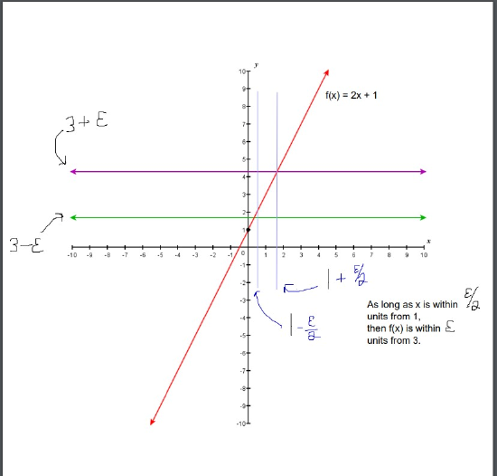
Figure \(\PageIndex{2}\): demonstrates our epsilon-delta setup for \(\displaystyle \lim_{x→1}(2x+1)=3\).
After removing all the remarks, here is a final version of the proof:
Let \(ε>0\).
Choose \(δ=ε/2\).
Assume \(0<|x−1|<δ\).
In other words:
\(0<|x−1|<\frac{ε}{2}\),
so \(-\frac{ε}{2}<x−1<\frac{ε}{2}\),
then \(-ε<2x−2<ε\)
then |\(2x−2|<ε\),
then |(\(2x+1)−3\)|<ε
Thus, if \(0<|x−1|<δ\), then |(\(2x+1)−3\)|<ε.
Therefore, by the definition of limit, \(\displaystyle \lim_{x→1}(2x+1)=3\).
The following Problem-Solving Strategy summarizes the type of proof we worked out in Example \(\PageIndex{1}\).
Problem-Solving Strategy: Proving That \(\displaystyle \lim_{x→a}f(x)=L\) for a Specific Function \(f(x)\)
- Let’s begin the proof with the following statement: Let \(ε>0\).
- Next, we need to obtain our choice for \(δ\) (use the Analysis Doodle). The Analysis Doodle is scratch work done to find our choice for \(δ\). Always put it on a separate page, or in a box marked "Scratch Work". Make the following statement, filling in the blank with our discovered choice of δ: Choose \(δ=\)_______.
- The next statement in the proof should be (at this point, we fill in our given value for a): Assume \(0<|x−a|<δ\).
- Starting with \(0<|x−a|<δ\), use our choice of \(δ\) and algebra to lead to \(|f(x)−L|<ε\), where \(f(x)\) and L are our function \(f(x)\) and our limit L.
- This shows (and you should state) if \(0<|x−a|<δ\), then \(|f(x)−L|<ε\).
- We conclude our proof with the statement: Therefore, by the definition of limit, \(\displaystyle \lim_{x→a}f(x)=L\).
Example \(\PageIndex{2}\): Proving a Statement about a Limit
Complete the proof that \(\displaystyle \lim_{x→−1}(4x+1)=−3\) by filling in the blanks.
Let _____.
Choose \(δ=\)_______.
Assume \(0<\)|\(x\)−_______|\(<δ\).
In other words, |\(x\)−_______|\(<\) _______, then _______________ then ________________ then _______________ ... then __________\(<ε\).
Thus, if ____________________________, then ________________.
Therefore, by _______________________________ _____________________________.
Solution
We begin by filling in the blanks where the choices are specified by the definition. Thus, we have
Let ε\(>0\).
SCRATCH WORK:
Choose \(δ\)= ??.
Here is our Analysis Doodle:
We want \(|4x+1 -(-3)|\) to be less than \(ε\), if \(0<\)|\(x−(−1)\)|\(<δ\).
So, we set \(|4x+1 -(-3)|<ε \) and fiddle around to get \(x−(−1)\) inside the absolute value.
\(|4x+1 -(-3)|<ε \) implies \(-ε<4x+4<ε \) implies \(-\frac{ε}{4}<x+1<\frac{ε}{4} \) implies \(|x+1|<\frac{ε}{4} \)
Thus we see that we should choose \(δ=\frac{ε}{4}\).
We now complete the final write-up of the proof:
Let ε\(>0\).
Choose \(δ=\frac{ε}{4}\).
Assume \(0<\)|\(x−(−1)\)|\(<δ\) (or equivalently, \(0<\)|\(x+1\)|\(<δ\).)
In other words:
\(0<|x+1|<\frac{ε}{4}\),
so \(-\frac{ε}{4}<x+1<\frac{ε}{4}\),
then \(-ε<4x+4<ε\)
then |\(4x+4|<ε\),
then |(\(4x+1)−(-3)\)|<ε
Thus, if \(0<|x−(-1)|<δ\), then |(\(4x+1)−(-3)\)|<ε.
Therefore, by the definition of limit, \(\displaystyle \lim_{x→-1}(4x+1)=-3\).
![]() \(\PageIndex{1}\)
\(\PageIndex{1}\)
Complete the proof that \(\displaystyle \lim_{x→2}(3x−2)=4\) by filling in the blanks. (Your Analysis Doodle is NOT written in the actual proof.)
Let _______.
Choose \(δ\) =_______.
Assume \(0<\)|\(x−\)____|\(<\)____.
In other words, |\(x\)−_______|\(<\) _______, then _______________ then ________________ then _______________ ... then __________\(<ε\).
Thus, if ____________________________, then ________________.
Therefore, by _______________________________ _____________________________.
- Hint
-
Follow the outline in the Problem-Solving Strategy that we worked out in full in Example \(\PageIndex{2}\).
- Answer
-
Let ε\(>0\); choose \(δ=\frac{ε}{3}\); assume \(0<|x−2|<δ\).
In other words:
\(0<|x - 2|<\frac{ε}{3}\),
so \(-\frac{ε}{3}<x - 2<\frac{ε}{3}\),
then \(-ε<3x - 6<ε\)
then |\(3x - 6|<ε\),
then |(\(3x - 2)−4\)|<ε
Thus, if \(0<|x−2|<δ\), then |(\(3x - 2)−4\)|<ε.
Therefore, by the definition of limit, \(\displaystyle \lim_{x→2}3x−2=4\).
Precise Definitions for Limits at Infinity
Earlier, we used the terms arbitrarily close, arbitrarily large, and sufficiently large to define limits at infinity informally. Although these terms provide accurate descriptions of limits at infinity, they are not precise mathematically. Here are more formal definitions of limits at infinity. We then look at how to use these definitions to prove results involving limits at infinity.
Definition: Limit at Infinity (Formal)
We say a function \(f\) has a limit at infinity, if there exists a real number \(L\) such that for all \(ε>0\), there exists \(N>0\) such that
\[|f(x)−L|<ε\]
for all \(x>N.\) in that case, we write
\[\lim_{x→∞}f(x)=L\]
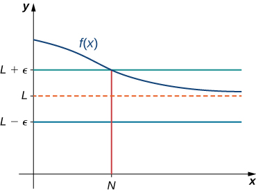
Figure \(\PageIndex{3}\): For a function with a limit at infinity, for all \(x>N, |f(x)−L|<ε.\)
Earlier in this section, we used graphical evidence in Figure and numerical evidence in Table to conclude that \(\lim_{x→∞}(\frac{2+1}{x})=2\). Here we use the formal definition of limit at infinity to prove this result rigorously.
Example \(\PageIndex{3}\):
Use the formal definition of limit at infinity to prove that \(\displaystyle \lim_{x→∞}2+\frac{1}{x}=2\).
Solution
Let \(ε>0.\) Let \(N=\frac{1}{ε}\). Therefore, for all \(x>N\), we have
\[|2+\frac{1}{x}−2|=|\frac{1}{x}|=\frac{1}{x}<\frac{1}{N}=ε\]
Therefore, \(\displaystyle \lim_{x→∞}2+\frac{1}{x}=2\).
![]() \(\PageIndex{2}\)
\(\PageIndex{2}\)
Use the formal definition of limit at infinity to prove that \(\displaystyle \lim_{x→∞}3−\frac{1}{x^2}=3\).
- Hint
-
Let \(N=\frac{1}{\sqrt{ε}}\).
- Answer
-
Let \(ε>0.\) Let \(N=\frac{1}{\sqrt{ε}}\). Therefore, for all \(x>N,\) we have
\(∣3−\frac{1}{x^2}−3∣=\frac{1}{x^2}<\frac{1}{N^2}=ε\)
Therefore, \(\displaystyle \lim_{x→∞}(3−\frac{1}{x^2})=3.\)
We now turn our attention to a more precise definition for an infinite limit at infinity.
Definition: Infinite Limit at Infinity (Formal)
We say a function \(f\) has an infinite limit at infinity and write
\(\displaystyle \lim_{x→∞}f(x)=∞\)
if for all \(M>0,\) there exists an \(N>0\) such that
\(f(x)>M\)
for all \(x>N\) (see Figure).
We say a function has a negative infinite limit at infinity and write
\(\displaystyle \lim_{x→∞}f(x)=−∞\)
if for all \(M<0\), there exists an \(N>0\) such that
\(f(x)<M\)
for all \(x>N\).
Similarly we can define limits as \(x→−∞.\)
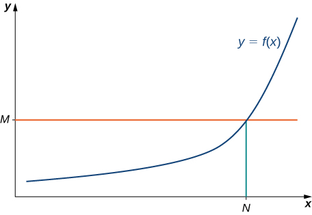
Figure \(\PageIndex{4}\): For a function with an infinite limit at infinity, for all \(x>N, f(x)>M.\)
Here we use the formal definition of infinite limit at infinity to prove \(\displaystyle \lim_{x→∞}x^3=∞\).
Example \(\PageIndex{4}\):
Use the formal definition of infinite limit at infinity to prove that \(\displaystyle \lim_{x→∞}x^3=∞.\)
Doodle Analysis: For some \(M>0\), we need an \(N\) so that if \(x>N\), we get \(x^3>M\).
Start with \(x^3>M\), and solve for \(x\). \(x>\sqrt[3]{M}\). So, as long as \(x>\sqrt[3]{M}\), then \(x^3>M\). So, choose \(N=\sqrt[3]{M}\).
Proof:
Let \(M>0.\) Choose \(N=\sqrt[3]{M}\). Then, for all \(x>N\), we have
\(x^3>N^3=(\sqrt[3]{M})^3=M.\)
Therefore, by the definition of limit, \(\displaystyle \lim_{x→∞}x^3=∞\).
![]() \(\PageIndex{3}\)
\(\PageIndex{3}\)
Use the formal definition of infinite limit at infinity to prove that \(\displaystyle \lim_{x→∞}3x^2=∞.\)
- Hint
-
Let \(N=\sqrt{\frac{M}{3}}\).
- Answer
-
Let \(M>0.\) Let \(N=\sqrt{\frac{M}{3}})\). Then, for all \(x>N,\) we have
\(3x^2>3N^2=3(\sqrt{\frac{M}{3}})^22=\frac{3M}{3}=M\)
One-Sided Limits
Just as we first gained an intuitive understanding of limits and then moved on to a more rigorous definition of a limit, we now revisit one-sided limits. To do this, we modify the epsilon-delta definition of a limit to give formal epsilon-delta definitions for limits from the right and left at a point. These definitions only require slight modifications from the definition of the limit. In the definition of the limit from the right, the inequality \(0<x−a<δ\) replaces \(0<|x−a|<δ\), which ensures that we only consider values of x that are greater than (to the right of) a. Similarly, in the definition of the limit from the left, the inequality \(−δ<x−a<0\) replaces \(0<|x−a|<δ\), which ensures that we only consider values of x that are less than (to the left of) a.
Definition
Limit from the Right: Let \(f(x)\) be defined over an open interval of the form \((a,b)\) where \(a<b\). Then
\[\lim_{x→a^+}f(x)=L\]
if for every \(ε>0\), there exists a \(δ>0\), such that if \(0<x−a<δ\), then \(|f(x)−L|<ε\).
Limit from the Left: Let \(f(x)\) be defined over an open interval of the form \((b,c)\) where \(b<c\). Then,
\[\lim_{x→c^−}f(x)=L\]
if for every \(ε>0\), there exists a \(δ>0\) such that if \( −δ<x−c<0\), then \(|f(x)−L|<ε\).
Example \(\PageIndex{5}\): Proving a Statement about a Limit From the Right
Prove that
\[lim_{x→4^+}\sqrt{x−4}=0.\]
Solution
Let ε>0.
Choose \(δ=ε^2\). Since we ultimately want \(∣\sqrt{x−4}−0∣<ε\), we manipulate this inequality to get \(\sqrt{x−4}<ε\) or, equivalently, \(0<x−4<ε^2\), making \(δ=ε^2\) a clear choice.
Assume \(0<x−4<δ\). Thus, \(0<x−4<ε^2\). Hence, \(0<\sqrt{x−4}<ε\). Finally, \(∣\sqrt{x−4}−0∣<ε\). Therefore, \(\displaystyle \lim_{x→4^+}\sqrt{x−4}=0\).
![]() \(\PageIndex{4}\)
\(\PageIndex{4}\)
Find \(δ\) corresponding to \(ε\) for a proof that \(\displaystyle \lim_{x→1^−}\sqrt{1−x}=0\).
- Hint
-
Sketch the graph and use Example as a solving guide.
- Answer
-
\(δ=ε^2\)
Infinite Limits
We conclude the process of converting our intuitive ideas of various types of limits to rigorous formal definitions by pursuing a formal definition of infinite limits. To have \(\displaystyle \lim_{x→a}f(x)=+∞\), we want the values of the function \(f(x)\) to get larger and larger as x approaches a. Instead of the requirement that \(|f(x)−L|<ε\) for arbitrarily small \(ε\) when \(0<|x−a|<δ\) for small enough \(δ\), we want \(f(x)>M\) for arbitrarily large positive M when \(0<|x−a|<δ\) for small enough \(δ\). Figure illustrates this idea by showing the value of \(δ\) for successively larger values of M.
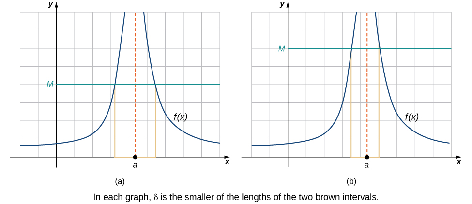
Figure \(\PageIndex{5}\): These graphs plot values of \(δ\) for M to show that \(\displaystyle \lim_{x→a}f(x)=+∞\).
Definition
Let \(f(x)\) be defined for all \(x≠a\) in an open interval containing a. Then, we have an infinite limit
\[\lim_{x→a}f(x)=+∞\]
if for every \(M>0\), there exists \(δ>0\) such that if \(0<|x−a|<δ\), then \(f(x)>M\).
Let \(f(x)\) be defined for all \(x≠a\) in an open interval containing a. Then, we have a negative infinite limit
\[\lim_{x→a}f(x)=−∞\]
if for every \(M>0\), there exists \(δ>0\) such that if \(0<|x−a|<δ\), then \(f(x)<−M\).
Advanced Topics
Here are some more complex problems using the precise definition of limit. Feel free to look these over; however, you are not required to know the remaining topics in this section.
In Examples \(\PageIndex{1}\) and \(\PageIndex{2}\), the proofs were fairly straightforward, since the functions with which we were working were linear. In Example, we see how to modify the proof to accommodate a nonlinear function.
Example \(\PageIndex{6}\):Proving a Statement about the Limit of a Quadratic Function
Let’s use our outline from the Problem-Solving Strategy:
1. Let \(ε>0\).
2. Choose \(δ=min\){\(1,ε/5\)}. This choice of \(δ\) may appear odd at first glance, but it was obtained by taking a look at our ultimate desired inequality: ∣\((x^2−2x+3)−6\)∣\(<ε\). This inequality is equivalent to \(|x+1|⋅|x−3|<ε\). At this point, the temptation simply to choose \(δ=\frac{ε}{x−3}\) is very strong. Unfortunately, our choice of \(δ\) must depend on ε only and no other variable. If we can replace \(|x−3|\) by a numerical value, our problem can be resolved. This is the place where assuming \(δ≤1\) comes into play. The choice of \(δ≤1\) here is arbitrary. We could have just as easily used any other positive number. In some proofs, greater care in this choice may be necessary. Now, since \(δ≤1\) and \(|x+1|<δ≤1\), we are able to show that \(|x−3|<5\). Consequently, \(|x+1|⋅|x−3|<|x+1|⋅5\). At this point we realize that we also need \(δ≤ε/5\). Thus, we choose \(δ=min\){\(1,ε/5\)}.
3. Assume \(0<|x+1|<δ\). Thus,
\[|x+1|<1\] and \[|x+1|<\frac{ε}{5}.\]
Since \(|x+1|<1\), we may conclude that \(−1<x+1<1\). Thus, by subtracting 4 from all parts of the inequality, we obtain \(−5<x−3<−1\). Consequently, \(|x−3|<5\). This gives us
\[∣(x^2−2x+3)−6∣=|x+1|⋅|x−3|<\frac{ε}{5}⋅5=ε.\]
Therefore,
\[\displaystyle \lim_{x→−1}(x^2−2x+3)=6.\]
![]() \(\PageIndex{5}\)
\(\PageIndex{5}\)
Complete the proof that \(\displaystyle \lim_{x→1}x^2=1\).
Let \(ε>0\); choose \(δ=min\){\(1,ε/3\)}; assume \(0<|x−1|<δ\).
Since \(|x−1|<1\), we may conclude that \(−1<x−1<1\). Thus, \(1<x+1<3\). Hence, \(|x+1|<3\).
- Hint
-
Use Example as a guide.
- Answer
-
\(∣x^2−1∣=|x−1|⋅|x+1|<ε/3⋅3=ε\)
Proving Limit Laws
We now demonstrate how to use the epsilon-delta definition of a limit to construct a rigorous proof of one of the limit laws. The triangle inequality is used at a key point of the proof, so we first review this key property of absolute value.
Definition
The triangle inequality states that if a and b are any real numbers, then \(|a+b|≤|a|+|b|\).
proof
We prove the following limit law: If \(\displaystyle \lim_{x→a}f(x)=L\) and \(\displaystyle \lim_{x→a}g(x)=M\), then \(\displaystyle \lim_{x→a}(f(x)+g(x))=L+M\).
Let \(ε>0\).
Choose \(δ_1>0\) so that if \(0<|x−a|<δ_1\), then \(|f(x)−L|<ε/2\).
Choose \(δ_2>0\) so that if \(0<|x−a|<δ_2\), then \(|g(x)−M|<ε/2\).
Choose \(δ=min\){\(δ_1,δ_2\)}.
Assume \(0<|x−a|<δ\).
Thus,
\(0<|x−a|<δ_1\) and \(0<|x−a|<δ_2\).
Hence,
\(|(f(x)+g(x))−(L+M)|=|(f(x)−L)+(g(x)−M)|\)
\(≤|f(x)−L|+|g(x)−M|\)
\(<\frac{ε}{2}+\frac{ε}{2}=ε\).
□
We now explore what it means for a limit not to exist. The limit \(\displaystyle \lim_{x→a}f(x)\) does not exist if there is no real number L for which \(\displaystyle \lim_{x→a}f(x)=L\). Thus, for all real numbers L, \(\displaystyle \lim_{x→a}f(x)≠L\). To understand what this means, we look at each part of the definition of \(\displaystyle \lim_{x→a}f(x)=L\) together with its opposite. A translation of the definition is given in Table.
| Definition | Opposite |
|---|---|
| 1. For every \(ε>0\), | 1. There exists \(ε>0\) so that |
| 2. there exists a \(δ>0\), so that | 2. for every \(δ>0\), |
| 3. if \(0<|x−a|<δ\), then \(|f(x)−L|<ε\). | 3. There is an x satisfying \(0<|x−a|<δ\) so that \(|f(x)−L|≥ε\). |
Finally, we may state what it means for a limit not to exist. The limit \(\displaystyle \lim_{x→a}f(x)\) does not exist if for every real number L, there exists a real number \(ε>0\) so that for all \(δ>0\), there is an x satisfying \(0<|x−a|<δ\), so that \(|f(x)−L|≥ε\). Let’s apply this in Example to show that a limit does not exist.
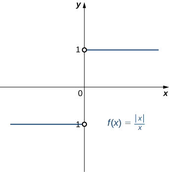
Example \(\PageIndex{7}\): Showing That a Limit Does Not Exist
Show that \(\displaystyle \lim_{x→0}\frac{|x|}{x}\) does not exist. The graph of \(f(x)=|x|/x\) is shown here:
Solution
Suppose that L is a candidate for a limit. Choose \(ε=1/2\).
Let \(δ>0\). Either \(L≥0\) or \(L<0\). If \(L≥0\), then let \(x=−δ/2\).
Thus,
\(|x−0|=∣−\frac{δ}{2}−0∣=\frac{δ}{2}<δ\)
and
\(∣\frac{∣−\frac{δ}{2}∣}{−\frac{δ}{2}}−L∣=|−1−L|=L+1≥1>\frac{1}{2}=ε\).
On the other hand, if \(L<0\), then let \(x=δ/2\). Thus,
\(|x−0|=∣\frac{δ}{2}−0∣=\frac{δ}{2}<δ\)
and
\(∣\frac{∣\frac{δ}{2}∣}{\frac{δ}{2}}−L∣=|1−L|=|L|+1≥1>\frac{1}{2}=ε\).
Thus, for any value of L, \(\displaystyle \lim_{x→0}\frac{|x|}{x}≠L.\)
Key Concepts
- The intuitive notion of a limit may be converted into a rigorous mathematical definition known as the epsilon-delta definition of the limit.
- The epsilon-delta definition may be used to prove statements about limits.
- The epsilon-delta definition of a limit may be modified to define one-sided limits.
Glossary
- epsilon-delta definition of the limit
- \(\displaystyle \lim_{x→a}f(x)=L\) if for every \(ε>0\), there exists a \(δ>0\) such that if \(0<|x−a|<δ\), then \(|f(x)−L|<ε\)
- triangle inequality
- If a and b are any real numbers, then \(|a+b|≤|a|+|b|\)
Contributors
Gilbert Strang (MIT) and Edwin “Jed” Herman (Harvey Mudd) with many contributing authors. This content by OpenStax is licensed with a CC-BY-SA-NC 4.0 license. Download for free at http://cnx.org.