NEW 2.3E: Limit Laws

2.3: The Limit Laws

In the following exercises, use the limit laws to evaluate each limit. Justify each step by indicating the appropriate limit law(s).

1) $lim_{x→0}(4x^2−2x+3)$

Solution: Use constant multiple law and difference law:

$lim_{x→0}(4x^2−2x+3)=4lim_{x→0}x^2−2lim_{x→0}x+lim_{x→0}3=3$

2) $lim_{x→1}\frac{x^3+3x^2+5}{4−7x}$

3) $lim_{x→−2}\sqrt{x^2−6x+3}$

Solution: Use root law: $lim_{x→−2}\sqrt{x^2−6x+3}=\sqrt{lim_{x→−2}(x2−6x+3)}=\sqrt{19}$

4) $lim_{x→−1}(9x+1)^2$

In the following exercises, use direct substitution to evaluate each limit.

5) $lim_{x→7}x^2)$

Solution: 49

6) $lim_{x→−2}(4x^2−1)$

7) $lim_{x→0}\frac{1}{1+sinx}$

Solution: 1

8) $lim_{x→2}e^{2x−x^2}$

9) $lim_{x→1}\frac{2−7x}{x+6}$

Solution: $−\frac{5}{7}$

10) $lim_{x→3}lne^{3x}$

In the following exercises, use direct substitution to show that each limit leads to the indeterminate form $0/0$. Then, evaluate the limit.

11) $lim_{x→4}\frac{x^2−16}{x−4}$

Solution:$lim_{x→4}\frac{x^2−16}{x−4}=\frac{16−16}{4−4}=\frac{0}{0}; then, lim_{x→4}\frac{x^2−16}{x−4}= lim_{x→4}\frac{(x+4)(x−4)}{x−4}=8$

12) $lim_{x→2}\frac{x−2}{x^2−2x}$

13) $lim_{x→6}\frac{3x−18}{2x−12}$

Solution: $lim_{x→6}\frac{3x−18}{2x−12}=\frac{18−18}{12−12}=\frac{0}{0}; then, lim_{x→6}\frac{3x−18}{2x− 12}=lim_{x→6}\frac{3(x−6)}{2(x−6)}=\frac{3}{2}$

14) $lim_{h→0}\frac{(1+h)^2−1}{h}$

15) $lim_{t→9}\frac{t−9}{\sqrt{t−3}}$

Solution: $lim_{x→9}\frac{t−9}{\sqrt{t}−3}=\frac{9−9}{3−3}=\frac{0}{0}; then, lim_{t→9}\frac{t−9}{\sqrt{t}−3} =lim_{t→9}\frac{t−9}{\sqrt{t}−3}\frac{\sqrt{t}+3}{\sqrt{t}+3}=lim_{t→9}(\sqrt{t}+3)=6$

16) $lim_{h→0}\frac{\frac{1}{a+h}−\frac{1}{a}}{h}$, where a is a real-valued constant

17) $lim_{θ→π}\frac{sinθ}{tanθ}$

Solution: $lim_{θ→π}\frac{sinθ}{tanθ}=\frac{sinπ}{tanπ}=\frac{0}{0}; then, lim_{θ→π}\frac{sinθ}{tanθ}=lim_{θ→ π}\frac{sinθ}{\frac{sinθ}{cosθ}}=lim_{θ→π}cosθ=−1$

18) $lim_{x→1}\frac{x^3−1}{x^2−1}$

19) $lim_{x→1/2}\frac{2x^2+3x−2}{2x−1}$

Solution: $lim_{x→1/2}\frac{2x^2+3x−2}{2x−1}=\frac{\frac{1}{2}+\frac{3}{2}−2}{1−1}=\frac{0}{0}; then, lim_{x→ 1/2}\frac{2x^2+3x−2}{2x−1}=lim_{x→1/2}frac{(2x−1)(x+2)}{2x−1}=\frac{5}{2}$

20) $lim_{x→−3}\frac{\sqrt{x+4}−1}{x+3}$

In the following exercises, use direct substitution to obtain an undefined expression. Then, use the method of Example to simplify the function to help determine the limit.

21) $lim_{x→−2^−}\frac{2x^2+7x−4}{x^2+x−2}$

Solution: −∞

22) $lim_{x→−2^+}\frac{2x^2+7x−4}{x^2+x−2}$

23) $lim_{x→1^−}\frac{2x^2+7x−4}{x^2+x−2}$

Solution: −∞

24) $lim_{x→1^+}\frac{2x^2+7x−4}{x^2+x−2}$

In the following exercises, assume that $lim_{x→6}f(x)=4,lim_{x→6}g(x)=9$, and $lim_{x→6}h(x)=6$. Use these three facts and the limit laws to evaluate each limit

25) $lim_{x→6}2f(x)g(x)$

Solution: $lim_{x→6}2f(x)g(x)=2lim_{x→6}f(x)lim_{x→6}g(x)=72$

26) $lim_{x→6}\frac{g(x)−1}{f(x)}$

27) $lim_{x→6}(f(x)+\frac{1}{3}g(x))$

Solution: $lim_{x→6}(f(x)+\frac{1}{3}g(x))=lim_{x→6}f(x)+\frac{1}{3}lim_{x→6}g(x)=7$\

28) $lim_{x→6}\frac{(h(x))^3}{2}$

29) $lim_{x→6}\sqrt{g(x)−f(x)}$

Solution: $lim_{x→6}\sqrt{g(x)−f(x)}=\sqrt{lim_{x→6}g(x)−lim_{x→6}f(x)}=\sqrt{5}$

30) $lim_{x→6}x⋅h(x)$

31) $lim_{x→6}[(x+1)⋅f(x)]$

Solution: $lim_{x→6}[(x+1)f(x)]=(lim_{x→6}(x+1))(lim_{x→6}f(x))=28$

32) $lim_{x→6}(f(x)⋅g(x)−h(x))$

[T] In the following exercises, use a calculator to draw the graph of each piecewise-defined function and study the graph to evaluate the given limits.

33) $f(x)=\begin{cases}x2 & x≤3,\\ x+4 & x>3\end{cases}$

1. a. $lim_{x→3^−}f(x)$
2. b. $lim_{x→3^+}f(x)$

Solution:

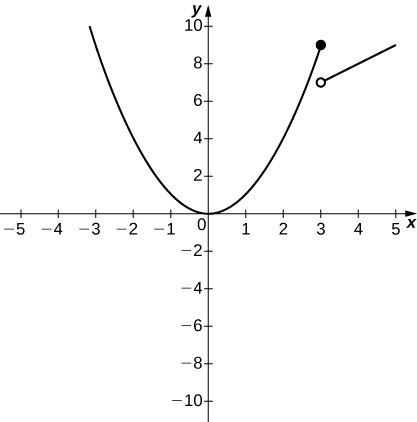
a. 9; b. 7

34) $g(x)=\begin{cases}x^3−1 & x≤0\\1 & x>0\end{cases}$

1. a. $lim_{x→0^−}g(x)$
2. b. $lim_{x→0^+}g(x)$

35) $h(x)=\begin{cases}x^2−2x+1 & x<2x≥2\\3−x & x≥2\end{cases}$

1. a. $lim_{x→2^−}h(x)$
2. b. $lim_{x→2^+}h(x)$

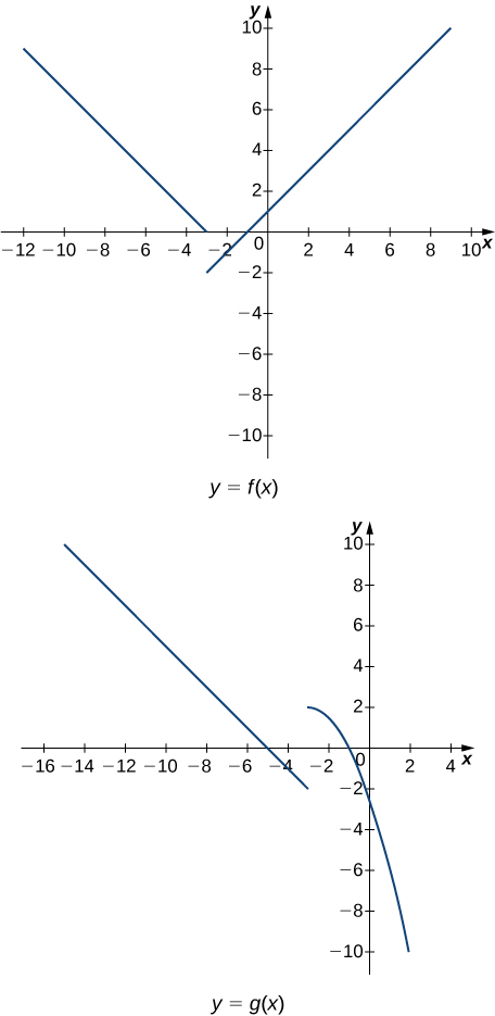
In the following exercises, use the following graphs and the limit laws to evaluate each limit.

36) $lim_{x→−3^+}(f(x)+g(x))$

37) $lim_{x→−3^−}(f(x)−3g(x))$

Solution: $lim_{x→−3^−}(f(x)−3g(x))=lim_{x→−3^−}f(x)−3lim_{x→−3^−}g(x)=0+6=6$

38) $lim_{x→0}\frac{f(x)g(x)}{3}$

39) $lim_{x→−5}\frac{2+g(x)}{f(x)}$

Solution: $lim_{x→−5}\frac{2+g(x)}{f(x)}=\frac{2+(lim_{x→−5}g(x))}{lim_{x→−5}f(x)}=\frac{2+0}{2}=1$

40) $lim_{x→1}(f(x))^2$

41) $lim_{x→1}\sqrt{f(x)−g(x)}$

Solution: $lim_{x→1}\sqrt[3]{f(x)−g(x)}=\sqrt[3]{lim_{x→1}f(x)−lim_{x→1}g(x)}=\sqrt[3]{2+5}=\sqrt[3]{7}$

42) $lim_{x→−7}(x⋅g(x))$

43) $lim_{x→−9}[x⋅f(x)+2⋅g(x)]$

Solution: $lim_{x→−9}(xf(x)+2g(x))=(lim_{x→−9}x)(lim_{x→−9}f(x))+2lim_{x→−9}(g(x))=(−9)(6)+2(4)=−46$

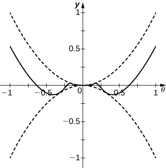
For the following problems, evaluate the limit using the squeeze theorem. Use a calculator to graph the functions $f(x),g(x)$, and $h(x)$ when possible.

44) [T] True or False? If $2x−1≤g(x)≤x^2−2x+3$, then $lim_{x→2}g(x)=0$.

45) [T] \(lim_{θ→0}θ^2cos(\frac{1}{θ})

Solution: The limit is zero.

46) $lim_{x→0}f(x)$, where $f(x)=\begin{cases}0 & x rational\\ x^2 & x irrrational\end{cases}$

47) [T] In physics, the magnitude of an electric field generated by a point charge at a distance r in vacuum is governed by Coulomb’s law: $E(r)=\frac{q}{4πε0_r^2}$, where E represents the magnitude of the electric field, q is the charge of the particle, r is the distance between the particle and where the strength of the field is measured, and \frac{1}{4πε_0} is Coulomb’s constant: $8.988×109N⋅m^2/C^2$.

a. Use a graphing calculator to graph $E(r)$ given that the charge of the particle is $q=10^{−10}$.

b. Evaluate $lim_{r→0^+}E(r)$. What is the physical meaning of this quantity? Is it physically relevant? Why are you evaluating from the right?

Solution: a

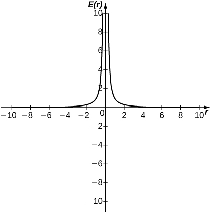
b. ∞. The magnitude of the electric field as you approach the particle q becomes infinite. It does not make physical sense to evaluate negative distance.

48) [T] The density of an object is given by its mass divided by its volume: $ρ=m/V.$

a. Use a calculator to plot the volume as a function of density $(V=m/ρ)$, assuming you are examining something of mass 8 kg ($m=8$).

b. Evaluate $lim_{x→0^+}V(\rho)$ and explain the physical meaning.

2.4: Continuity

Chapter Review Exercises

True or False. In the following exercises, justify your answer with a proof or a counterexample.

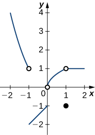
212) Using the graph, find each limit or explain why the limit does not exist.

a. $lim_{x→−1}f(x)$

b. $lim_{x→1}f(x)$

c. $lim_{x→0^+}f(x)$

d. $lim_{x→2}f(x)$

---

In the following exercises, evaluate the limit algebraically or explain why the limit does not exist.

213) $lim_{x→2}\frac{2x^2−3x−2}{x−2}$

Solution: 5

214) $lim_{x→0}3x^2−2x+4$

215) $lim_{x→3}\frac{x^3−2x^2−1}{3x−2}$

Solution: 8/7

216) $lim_{x→π/2}\frac{cotx}{cosx}$ This is covered in section 2.4

217) $lim_{x→−5}\frac{x^2+25}{x+5}$

Solution:DNE

218) $lim_{x→2}\frac{3x^2−2x−8}{x^2−4}$

219) $lim_{x→1}\frac{x^2−1}{x^3−1}$

Solution: 2/3

220) $lim_{x→1}\frac{x^2−1}{\sqrt{x}−1}$

221) $lim_{x→4}\frac{4−x}{\sqrt{x}−2}$

Solution: −4

222) $lim_{x→4}\frac{1}{\sqrt{x}−2}$

---

In the following exercises, use the squeeze theorem to prove the limit.

223) $lim_{x→0}x^2cos(2πx)=0$

Solution: Since $−1≤cos(2πx)≤1$, then $−x^2≤x^2cos(2πx)≤x^2$. Since $lim_{x→0}x^2=0=lim_{x→0}−x^2$, it follows that $lim_{x→0}x^2cos(2πx)=0$.

224) $lim_{x→0}x^3sin(\frac{π}{x})=0$