5.5E

5.5: Substitution

In the following exercises, find the antiderivative.

261) \(\displaystyle∫(x+1)^4dx\)

Answer:

\(\displaystyle\frac{1}{5}(x+1)^5+C\)

262) \(\displaystyle∫(x−1)^5dx\)

263) \(\displaystyle∫(2x−3)^{−7}dx\)

Answer:

\(\displaystyle−\frac{1}{12(3−2x)^6}+C\)

264) \(\displaystyle∫(3x−2)^{−11}dx\)

265) \(\displaystyle∫\frac{x}{\sqrt{x^2+1}}dx\)

Answer:

\(\displaystyle\sqrt{x^2+1}+C\)

266) \(\displaystyle∫\frac{x}{\sqrt{1−x^2}}dx\)

267) \(\displaystyle∫(x−1)(x^2−2x)^3dx\)

Answer:

\(\displaystyle\frac{1}{8}(x^2−2x)^4+C\)

268) \(\displaystyle∫(x^2−2x)(x^3−3x^2)^2dx\)

269) \(\displaystyle∫cos^3θdθ(Hint:cos^2θ=1−sin^2θ)\)

Answer:

\(\displaystylesinθ−\frac{sin^3θ}{3}+C\)

270) \(\displaystyle∫sin^3θdθ(Hint:sin^2θ=1−cos^2θ)\)

271) \(\displaystyle∫x(1−x)^{99}dx\)

Solution: \(\displaystyle\frac{(1−x)^{101}}{101}−\frac{(1−x)^{100}}{100}+C\)

272) \(\displaystyle∫t(1−t^2)^{10}dt\)

273) \(\displaystyle∫(11x−7)^{−3}dx\)

Answer:

\(\displaystyle−\frac{1}{22(7−11x^2)}+C\)

274) \(\displaystyle∫(7x−11)^4dx\)

275) \(\displaystyle∫cos^3θsinθdθ\)

Answer:

\(\displaystyle−\frac{cos^4θ}{4}+C\)

276) \(\displaystyle∫sin^3θdθ;u=cosθ (Hint:sin^2θ=1−cos^2θ)\)

(removed exercises 277- 280)

281) \(\displaystyle∫\frac{x^2}{(x^3−3)^2}dx\)

Answer:

\(\displaystyle−\frac{1}{3(x^3−3)}+C\)

In the following exercises, evaluate the definite integral.

292) \(\displaystyle∫^1_0x\sqrt{1−x^2}dx\)

293) \(\displaystyle∫^1_0\frac{x}{\sqrt{1+x^2}}dx\)

Answer:

\(\displaystyle u=1+x^2,du=2xdx,\frac{1}{2}∫^2_1u^{−1/2}du=\sqrt{2}−1\)

294) \(\displaystyle∫^2_0\frac{t}{\sqrt{5+t^2}}dt\)

295) \(\displaystyle∫^1_0\frac{t}{\sqrt{1+t^3}}dt\)

Answer:

\(\displaystyle u=1+t^3,du=3t^2,\frac{1}{3}∫^2_1u^{−1/2}du=\frac{2}{3}(\sqrt{2}−1)\)

296) \(\displaystyle∫^{π/4}_0sec^2θtanθdθ\)

297) \(\displaystyle∫^{π/4}_0\frac{sinθ}{cos^4θ}dθ\)

Answer:

\(\displaystyle u=cosθ,du=−sinθdθ,∫^1_{1/\sqrt{2}}u^{−4}du=\frac{1}{3}(2\sqrt{2}−1)\)

J5.5.1)

J5.5.2)

5.6: Integrals Involving Exponential and Logarithmic Functions

In the following exercises, compute each indefinite integral.

320) \(\displaystyle ∫e^{2x}dx\)

321) \(\displaystyle ∫e^{−3x}dx\)

Answer:

\(\displaystyle \frac{−1}{3}e^{−3x}+C\)

322) \(\displaystyle ∫2^xdx\)

323) \(\displaystyle ∫3^{−x}dx\)

Answer:

\(\displaystyle −\frac{3^{−x}}{ln3}+C\)

324) \(\displaystyle ∫\frac{1}{2x}dx\)

325) \(\displaystyle ∫\frac{2}{x}dx\)

Answer:

\(\displaystyle ln(x^2)+C\) or \(\displaystyle 2ln|x|+C\)

326) \(\displaystyle ∫\frac{1}{x^2}dx\)

327) \(\displaystyle ∫\frac{1}{\sqrt{x}}dx\)

Answer:

\(\displaystyle 2\sqrt{x}+C\)

In the following exercises, find each indefinite integral by using appropriate substitutions.

328) \(\displaystyle ∫\frac{lnx}{x}dx\)

329) \(\displaystyle ∫\frac{dx}{x(lnx)^2}\)

Answer:

\(\displaystyle −\frac{1}{lnx}+C\)

336) \(\displaystyle ∫xe^{−x^2}dx\)

337) \(\displaystyle ∫x^2e^{−x^3}dx\)

Answer:

\(\displaystyle \frac{−e^{−x^3}}{3}+C\)

338) \(\displaystyle ∫e^{sinx}cosxdx\)

339) \(\displaystyle ∫e^{tanx}sec^2xdx\)

Answer:

\(\displaystyle e^{tanx}+C\)

340) \(\displaystyle ∫e^{lnx}\frac{dx}{x}\)

341) \(\displaystyle ∫\frac{e^{ln(1−t)}}{1−t}dt\)

Answer:

\(\displaystyle t+C\)

In the following exercises, evaluate the definite integral.

355) \(\displaystyle ∫^2_1\frac{1+2x+x^2}{3x+3x^2+x^3}dx\)

Answer:

\(\displaystyle \frac{1}{3}ln(\frac{26}{7})\)

356) \(\displaystyle ∫^{π/4}_0tanxdx\)

357) \(\displaystyle ∫^{π/3}_0\frac{sinx−cosx}{sinx+cosx}dx\)

Answer:

\(\displaystyle ln(\sqrt{3}−1)\)

358) \(\displaystyle ∫^{π/2}_{π/6}cscxdx\)

359) \(\displaystyle ∫^{π/3}_{π/4}cotxdx\)

Answer:

\(\displaystyle \frac{1}{2}ln\frac{3}{2}\)

In the following exercises, integrate using the indicated substitution.

360) \(\displaystyle ∫\frac{x}{x−100}dx;u=x−100\)

361) \(\displaystyle ∫\frac{y−1}{y+1}dy;u=y+1\)

Answer:

\(\displaystyle y−2ln|y+1|+C\)

362) \(\displaystyle ∫\frac{1−x^2}{3x−x^3}dx;u=3x−x^3\)

363) \(\displaystyle ∫\frac{sinx+cosx}{sinx−cosx}dx;u=sinx−cosx\)

Answer:

\(\displaystyle ln|sinx−cosx|+C\)

364) \(\displaystyle ∫e^{2x}\sqrt{1−e^{2x}}dx;u=e^{2x}\)

365) \(\displaystyle ∫ln(x)\frac{\sqrt{1−(lnx)^2}}{x}dx;u=lnx\)

Answer:

\(\displaystyle −\frac{1}{3}(1−(lnx^2))^{3/2}+C\)

In the following exercises, \(\displaystyle f(x)≥0\) for \(\displaystyle a≤x≤b\). Find the area under the graph of \(\displaystyle f(x)\) between the given values a and b by integrating.

372) \(\displaystyle f(x)=\frac{log_{10}(x)}{x};a=10,b=100\)

373) \(\displaystyle f(x)=\frac{log_2(x)}{x};a=32,b=64\)

Answer:

\(\displaystyle \frac{11}{2}ln2\)

374) \(\displaystyle f(x)=2^{−x};a=1,b=2\)

375) \(\displaystyle f(x)=2^{−x};a=3,b=4\)

Answer:

\(\displaystyle \frac{1}{ln(65,536)}\)

376) Find the area under the graph of the function \(\displaystyle f(x)=xe^{−x^2}\) between \(\displaystyle x=0\) and \(\displaystyle x=5\).

377) Compute the integral of \(\displaystyle f(x)=xe^{−x^2}\) and find the smallest value of N such that the area under the graph \(\displaystyle f(x)=xe^{−x^2}\) between \(\displaystyle x=N\) and \(\displaystyle x=N+10\) is, at most, 0.01.

Answer:

\(\displaystyle ∫^{N+1}_Nxe^{−x^2}dx=\frac{1}{2}(e^{−N^2}−e^{−(N+1)^2}).\) The quantity is less than 0.01 when \(\displaystyle N=2\).

378) Find the limit, as N tends to infinity, of the area under the graph of \(\displaystyle f(x)=xe^{−x^2}\) between \(\displaystyle x=0\) and \(\displaystyle x=5\).

379) Show that \(\displaystyle ∫^b_a\frac{dt}{t}=∫^{1/a}_{1/b}\frac{dt}{t}\) when \(\displaystyle 0<a≤b\).

Answer:

\(\displaystyle ∫^b_a\frac{dx}{x}=ln(b)−ln(a)=ln(\frac{1}{a})−ln(\frac{1}{b})=∫^{1/a}_{1/b}\frac{dx}{x}\)

380) Suppose that \(\displaystyle f(x)>0\) for all x and that f and g are differentiable. Use the identity \(\displaystyle f^g=e^{glnf}\) and the chain rule to find the derivative of \(\displaystyle f^g\).

381) Use the previous exercise to find the antiderivative of \(\displaystyle h(x)=x^x(1+lnx)\) and evaluate \(\displaystyle ∫^3_2x^x(1+lnx)dx\).

Answer:

23

382) Show that if \(\displaystyle c>0\), then the integral of \(\displaystyle 1/x\) from ac to bc \(\displaystyle (0<a<b)\) is the same as the integral of \(\displaystyle 1/x\) from a to b.

The following exercises are intended to derive the fundamental properties of the natural log starting from the definition \(\displaystyle ln(x)=∫^x_1\frac{dt}{t}\), using properties of the definite integral and making no further assumptions.

383) Use the identity \(\displaystyle ln(x)=∫^x_1\frac{dt}{t}\) to derive the identity \(\displaystyle ln(\frac{1}{x})=−lnx\).

Solution: We may assume that \(\displaystyle x>1\),so \(\displaystyle \frac{1}{x}<1.\) Then, \(\displaystyle ∫^{1/x}_{1}\frac{dt}{t}\). Now make the substitution \(\displaystyle u=\frac{1}{t}\), so \(\displaystyle du=−\frac{dt}{t^2}\) and \(\displaystyle \frac{du}{u}=−\frac{dt}{t}\), and change endpoints: \(\displaystyle ∫^{1/x}_1\frac{dt}{t}=−∫^x_1\frac{du}{u}=−lnx.\)

384) Use a change of variable in the integral \(\displaystyle ∫^{xy}_1\frac{1}{t}dt\) to show that \(\displaystyle lnxy=lnx+lny\) for \(\displaystyle x,y>0\).

385) Use the identity \(\displaystyle lnx=∫^x_1\frac{dt}{x}\) to show that \(\displaystyle ln(x)\) is an increasing function of x on \(\displaystyle [0,∞)\), and use the previous exercises to show that the range of \(\displaystyle ln(x)\) is \(\displaystyle (−∞,∞)\). Without any further assumptions, conclude that \(\displaystyle ln(x)\) has an inverse function defined on \(\displaystyle (−∞,∞).\)

386) Pretend, for the moment, that we do not know that \(\displaystyle e^x\) is the inverse function of \(\displaystyle ln(x)\), but keep in mind that \(\displaystyle ln(x)\) has an inverse function defined on \(\displaystyle (−∞,∞)\). Call it E. Use the identity \(\displaystyle lnxy=lnx+lny\) to deduce that \(\displaystyle E(a+b)=E(a)E(b)\) for any real numbers a, b.

387) Pretend, for the moment, that we do not know that \(\displaystyle e^x\) is the inverse function of \(\displaystyle lnx\), but keep in mind that \(\displaystyle lnx\) has an inverse function defined on \(\displaystyle (−∞,∞)\). Call it E. Show that \(\displaystyle E'(t)=E(t).\)

Solution: \(\displaystyle x=E(ln(x)).\) Then, \(\displaystyle 1=\frac{E'(lnx)}{x}\) or \(\displaystyle x=E'(lnx)\). Since any number t can be written \(\displaystyle t=lnx\) for some x, and for such t we have \(\displaystyle x=E(t)\), it follows that for any \(\displaystyle t,E'(t)=E(t).\)

388) The sine integral, defined as \(\displaystyle S(x)=∫^x_0\frac{sint}{t}dt\) is an important quantity in engineering. Although it does not have a simple closed formula, it is possible to estimate its behavior for large x. Show that for \(\displaystyle k≥1,|S(2πk)−S(2π(k+1))|≤\frac{1}{k(2k+1)π}.\) (Hint: \(\displaystyle sin(t+π)=−sint\))

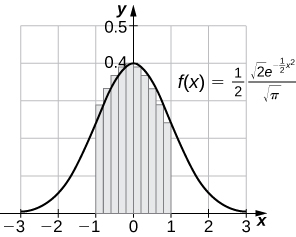
389) [T] The normal distribution in probability is given by \(\displaystyle p(x)=\frac{1}{σ\sqrt{2π}}e^{−(x−μ)^2/2σ^2}\), where σ is the standard deviation and μ is the average. The standard normal distribution in probability, \(\displaystyle p_s\), corresponds to \(\displaystyle μ=0\) and \(\displaystyle σ=1\). Compute the left endpoint estimates \(\displaystyle R_{10}\) and \(\displaystyle R_{100}\) of \(\displaystyle ∫^1_{−1}\frac{1}{\sqrt{2π}}e^{−x^{2/2}}dx.\)

Solution: \(\displaystyle R_{10}=0.6811,R_{100}=0.6827\)

390) [T] Compute the right endpoint estimates \(\displaystyle R_{50}\) and \(\displaystyle R_{100}\) of \(\displaystyle ∫^5_{−3}\frac{1}{2\sqrt{2π}}e^{−(x−1)^2/8}\).