5.7: Net Change

In this section, we use some basic integration formulas studied previously to solve some key applied problems. It is important to note that these formulas are presented in terms of indefinite integrals. Although definite and indefinite integrals are closely related, there are some key differences to keep in mind. A definite integral is either a number (when the limits of integration are constants) or a single function (when one or both of the limits of integration are variables). An indefinite integral represents a family of functions, all of which differ by a constant. As you become more familiar with integration, you will get a feel for when to use definite integrals and when to use indefinite integrals. You will naturally select the correct approach for a given problem without thinking too much about it. However, until these concepts are cemented in your mind, think carefully about whether you need a definite integral or an indefinite integral and make sure you are using the proper notation based on your choice.

Basic Integration Formulas

Recall the integration formulas given in [link] and the rule on properties of definite integrals. Let’s look at a few examples of how to apply these rules.

Example $\PageIndex{1}$: Integrating a Function Using the Power Rule

Use the power rule to integrate the function $∫^4_1\sqrt{t}(1+t)dt$.

Solution

The first step is to rewrite the function and simplify it so we can apply the power rule:

$$∫^4_1\sqrt{t}(1+t)dt=∫^4_1t^{1/2}(1+t)dt=∫^4_1(t^{1/2}+t^{3/2})dt.$$

Now apply the power rule:

$$∫^4_1(t^{1/2}+t^{3/2})dt=(\frac{2}{3}t^{3/2}+\frac{2}{5}t^{5/2})∣^4_1$$

$$=[\frac{2}{3}(4)^{3/2}+\frac{2}{5}(4)^{5/2}]−[\frac{2}{3}(1)^{3/2}+\frac{2}{5}(1)^{5/2}]=\frac{256}{15}.$$

Exercise $\PageIndex{1}$

Find the definite integral of $f(x)=x^2−3x$ over the interval $[1,3].$

Hint

Follow the process from Example to solve the problem.

Answer

$$−\frac{10}{3}$$

The Net Change Theorem

The net change theorem considers the integral of a rate of change. It says that when a quantity changes, the new value equals the initial value plus the integral of the rate of change of that quantity. The formula can be expressed in two ways. The second is more familiar; it is simply the definite integral.

Net Change Theorem

The new value of a changing quantity equals the initial value plus the integral of the rate of change:

$$F(b)=F(a)+∫^b_aF'(x)dx$$

or

$$∫^b_aF'(x)dx=F(b)−F(a).$$

Subtracting $F(a)$ from both sides of the first equation yields the second equation. Since they are equivalent formulas, which one we use depends on the application.

The significance of the net change theorem lies in the results. Net change can be applied to area, distance, and volume, to name only a few applications. Net change accounts for negative quantities automatically without having to write more than one integral. To illustrate, let’s apply the net change theorem to a velocity function in which the result is displacement.

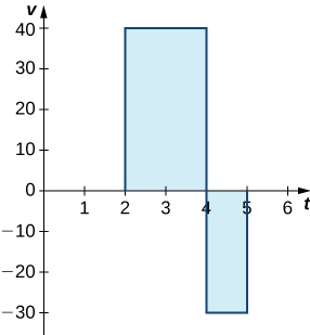
We looked at a simple example of this in The Definite Integral. Suppose a car is moving due north (the positive direction) at 40 mph between 2 p.m. and 4 p.m., then the car moves south at 30 mph between 4 p.m. and 5 p.m. We can graph this motion as shown in Figure.

Figure $\PageIndex{1}$: The graph shows speed versus time for the given motion of a car.

Just as we did before, we can use definite integrals to calculate the net displacement as well as the total distance traveled. The net displacement is given by

$$∫^5_2v(t)dt=∫^4_240dt+∫^5_4−30dt=80−30=50.$$

Thus, at 5 p.m. the car is 50 mi north of its starting position. The total distance traveled is given by

$$∫^5_2|v(t)|dt=∫^4_240dt+∫^5_430dt=80+30=110.$$

Therefore, between 2 p.m. and 5 p.m., the car traveled a total of 110 mi.

To summarize, net displacement may include both positive and negative values. In other words, the velocity function accounts for both forward distance and backward distance. To find net displacement, integrate the velocity function over the interval. Total distance traveled, on the other hand, is always positive. To find the total distance traveled by an object, regardless of direction, we need to integrate the absolute value of the velocity function.

Example $\PageIndex{2}$: Finding Net Displacement

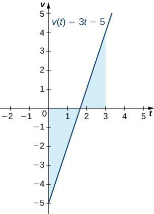
Given a velocity function $v(t)=3t−5$ (in meters per second) for a particle in motion from time $t=0$ to time $t=3,$ find the net displacement of the particle.

Solution

Applying the net change theorem, we have

$$∫^3_0(3t−5)dt=\frac{3t^2}{2}−5t∣^3_0=[\frac{3(3)^2}{2}−5(3)]−0=\frac{27}{2}−15=\frac{27}{2}−\frac{30}{2}=−\frac{3}{2}.$$

The net displacement is $−\frac{3}{2}$ m (Figure).

Figure $\PageIndex{2}$: The graph shows velocity versus time for a particle moving with a linear velocity function.

Example $\PageIndex{3}$: Finding the Total Distance Traveled

Use Example to find the total distance traveled by a particle according to the velocity function $v(t)=3t−5$ m/sec over a time interval $[0,3].$

Solution

The total distance traveled includes both the positive and the negative values. Therefore, we must integrate the absolute value of the velocity function to find the total distance traveled.

To continue with the example, use two integrals to find the total distance. First, find the t-intercept of the function, since that is where the division of the interval occurs. Set the equation equal to zero and solve for t. Thus,

$3t−5=0$

$3t=5$

$t=\frac{5}{3}.$

The two subintervals are $[0,\frac{5}{3}]$ and $[\frac{5}{3},3]$. To find the total distance traveled, integrate the absolute value of the function. Since the function is negative over the interval $[0,\frac{5}{3}]$, we have $|v(t)|=−v(t)$ over that interval. Over $[ \frac{5}{3},3]$, the function is positive, so $|v(t)|=v(t)$. Thus, we have

$∫^3_0|v(t)|dt=∫^{5/3}_0−v(t)dt+∫^3_{5/3}v(t)dt$

$=∫^{5/3}_05−3tdt+∫^3_{5/3}3t−5dt$

$=(5t−\frac{3t^2}{2})∣^{5/3}_0+(\frac{3t^2}{2}−5t)∣^3_{5/3}$

$=[5(\frac{5}{3})−\frac{3(5/3)^2}{2}]−0+[\frac{27}{2}−15]−[\frac{3(5/3)^2}{2}−\frac{25}{3}]$

$=\frac{25}{3}−\frac{25}{6}+\frac{27}{2}−15−\frac{25}{6}+\frac{25}{3}=\frac{41}{6}$.

So, the total distance traveled is $\frac{14}{6}$ m.

Exercise $\PageIndex{2}$

Find the net displacement and total distance traveled in meters given the velocity function $f(t)=\frac{1}{2}e^t−2$ over the interval $[0,2]$.

Hint

Follow the procedures from Example and Example. Note that $f(t)≤0$ for $t≤ln4$ and $f(t)≥0$ for $t≥ln4$.

Answer

Net displacement: $\frac{e^2−9}{2}≈−0.8055m;$ total distance traveled: $4ln4−7.5+\frac{e^2}{2}≈1.740 m$

Applying the Net Change Theorem

The net change theorem can be applied to the flow and consumption of fluids, as shown in Example.

Example $\PageIndex{4}$: How Many Gallons of Gasoline Are Consumed?

If the motor on a motorboat is started at $t=0$ and the boat consumes gasoline at the rate of $5−t^3$ gal/hr, how much gasoline is used in the first 2 hours?

Solution

Express the problem as a definite integral, integrate, and evaluate using the Fundamental Theorem of Calculus. The limits of integration are the endpoints of the interval [0,2]. We have

$$∫^2_0(5−t^3)dt=(5t−\frac{t^4}{4})∣^2_0=[5(2)−\frac{(2)^4}{4}]−0=10−\frac{16}{4}=6.$$

Thus, the motorboat uses 6 gal of gas in 2 hours.

Example $\PageIndex{5}$: Chapter Opener: Iceboats

As we saw at the beginning of the chapter, top iceboat racers can attain speeds of up to five times the wind speed. Andrew is an intermediate iceboater, though, so he attains speeds equal to only twice the wind speed.

Figure $\PageIndex{3}$: (credit: modification of work by Carter Brown, Flickr)

Suppose Andrew takes his iceboat out one morning when a light 5-mph breeze has been blowing all morning. As Andrew gets his iceboat set up, though, the wind begins to pick up. During his first half hour of iceboating, the wind speed increases according to the function $v(t)=20t+5.$ For the second half hour of Andrew’s outing, the wind remains steady at 15 mph. In other words, the wind speed is given by

$$v(t)=\begin{cases}20t+5& for 0≤t≤\frac{1}{2}\\15 & for \frac{1}{2}≤t≤1\end{cases}.$$

Recalling that Andrew’s iceboat travels at twice the wind speed, and assuming he moves in a straight line away from his starting point, how far is Andrew from his starting point after 1 hour?

Solution

To figure out how far Andrew has traveled, we need to integrate his velocity, which is twice the wind speed. Then

Distance =$∫^1_02v(t)dt.$

Substituting the expressions we were given for $v(t)$, we get

$∫^1_02v(t)dt=∫^{1/2}_02v(t)dt+∫^1_{1/2}2v(t)dt$

$=∫^{1/2}_02(20t+5)dt+∫^1_{1/3}2(15)dt$

$=∫^{1/2}_0(40t+10)dt+∫^1_{1/2}30dt$

$=[20t^2+10t]|^{1/2}_0+[30t]|^1_{1/2}$

$=(\frac{20}{4}+5)−0+(30−15)$

$=25.$

Andrew is 25 mi from his starting point after 1 hour.

Exercise $\PageIndex{3}$

Suppose that, instead of remaining steady during the second half hour of Andrew’s outing, the wind starts to die down according to the function $v(t)=−10t+15.$ In other words, the wind speed is given by

$v(t)=\begin{cases}20t+5 & for 0≤t≤\frac{1}{2}\\−10t+15& for\frac{1}{2}≤t≤1\end{cases}$.

Under these conditions, how far from his starting point is Andrew after 1 hour?

Hint

Don’t forget that Andrew’s iceboat moves twice as fast as the wind.

Answer

$17.5 mi$

Integrating Even and Odd Functions

We saw in Functions and Graphs that an even function is a function in which $f(−x)=f(x)$ for all x in the domain—that is, the graph of the curve is unchanged when x is replaced with −x. The graphs of even functions are symmetric about the y-axis. An odd function is one in which $f(−x)=−f(x)$ for all x in the domain, and the graph of the function is symmetric about the origin.

Integrals of even functions, when the limits of integration are from −a to a, involve two equal areas, because they are symmetric about the y-axis. Integrals of odd functions, when the limits of integration are similarly $[−a,a],$ evaluate to zero because the areas above and below the x-axis are equal.

Rule: Integrals of Even and Odd Functions

For continuous even functions such that $f(−x)=f(x),$

$$∫^a_{−a}f(x)dx=2∫^a_0f(x)dx.$$

For continuous odd functions such that $f(−x)=−f(x),$

$$∫^a_{−a}f(x)dx=0.$$

Example $\PageIndex{6}$: Integrating an Even Function

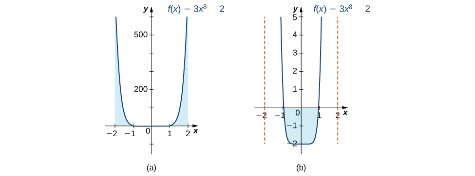
Integrate the even function $∫^2_{−2}(3x^8−2)dx$ and verify that the integration formula for even functions holds.

Solution

The symmetry appears in the graphs in Figure. Graph (a) shows the region below the curve and above the x-axis. We have to zoom in to this graph by a huge amount to see the region. Graph (b) shows the region above the curve and below the x-axis. The signed area of this region is negative. Both views illustrate the symmetry about the y-axis of an even function. We have

$∫^2_{−2}(3x^8−2)dx=(\frac{x^9}{3}−2x)∣^2_{−2}$

$=[\frac{(2)^9}{3}−2(2)]−[\frac{(−2)^9}{3}−2(−2)]$

$=(\frac{512}{3}−4)−(−\frac{512}{3}+4)$

$=\frac{1000}{3}$.

To verify the integration formula for even functions, we can calculate the integral from 0 to 2 and double it, then check to make sure we get the same answer.

$$∫^2_0(3x^8−2)dx=(\frac{x^9}{3}−2x)∣^2_0=\frac{512}{3}−4=\frac{500}{3}$$

Since $2⋅\frac{500}{3}=\frac{1000}{3},$ we have verified the formula for even functions in this particular example.

Figure $\PageIndex{4}$: Graph (a) shows the positive area between the curve and the x-axis, whereas graph (b) shows the negative area between the curve and the x-axis. Both views show the symmetry about the y-axis.

Example $\PageIndex{7}$: Integrating an Odd Function

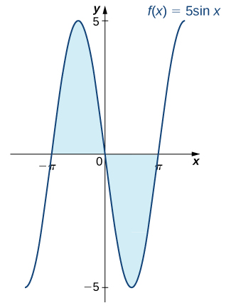
Evaluate the definite integral of the odd function $−5sinx$ over the interval $[−π,π].$

Solution

The graph is shown in Figure. We can see the symmetry about the origin by the positive area above the x-axis over $[−π,0]$, and the negative area below the x-axis over $[0,π].$ we have

$$∫^π_{−π}−5sinxdx=−5(−cosx)|^π_{−π}=5cosx|^π_{−π}=[5cosπ]−[5cos(−π)]=−5−(−5)=0.$$

Figure $\PageIndex{5}$:The graph shows areas between a curve and the x-axis for an odd function.

Exercise $\PageIndex{4}$

Integrate the function $∫^2_{−2}x^4dx.$

Hint

Integrate an even function.

Answer

$\dfrac{64}{5}$

Key Concepts

• The net change theorem states that when a quantity changes, the final value equals the initial value plus the integral of the rate of change. Net change can be a positive number, a negative number, or zero.
• The area under an even function over a symmetric interval can be calculated by doubling the area over the positive x-axis. For an odd function, the integral over a symmetric interval equals zero, because half the area is negative.

Key Equations

• Net Change Theorem

$F(b)=F(a)+∫^b_aF'(x)dx$ or $∫^b_aF'(x)dx=F(b)−F(a)$

Glossary

net change theorem

if we know the rate of change of a quantity, the net change theorem says the future quantity is equal to the initial quantity plus the integral of the rate of change of the quantity

Contributors

• Gilbert Strang (MIT) and Edwin “Jed” Herman (Harvey Mudd) with many contributing authors. This content by OpenStax is licensed with a CC-BY-SA-NC 4.0 license. Download for free at http://cnx.org.