1.5: Quadratic Solution Equations: Mold growth

Note

We examine mold growing on a solution of tea and sugar and find that models of this process lead to quadratic solution equations in contrast to the previous mathematical models which have exponential solution equations. Quadratic solution equations (equations of the form \(y = a t^{2} + b t + c\)) occur less frequently than do exponential solution equations in models of biological systems.

Shown in Figure 1.5.1 are some pictures taken of a mold colony growing on the surface of a mixture of tea and sugar. The pictures were taken at 10:00 each morning for 10 consecutive days. Assume that the area occupied by the mold is a reasonable measure of the size of the mold population. The grid lines are at \(2 mm\) intervals.

Explore 1.5.1 From the pictures, measure the areas of the mold for the days 2 and 6 and enter them into the table of Figure 1.5.2. The grid lines are at \(2 mm\) intervals, so that each square is \(4 mm^2\) . Check your additional data with points on the graph.

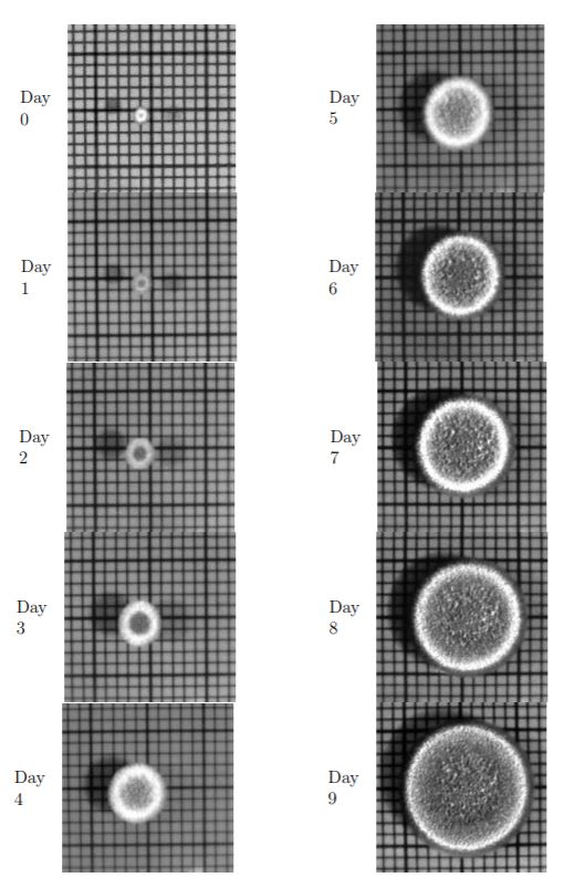
Figure \(\PageIndex{1}\): Pictures of a mold colony, taken on ten successive days. The grid lines are at 2 mm intervals.

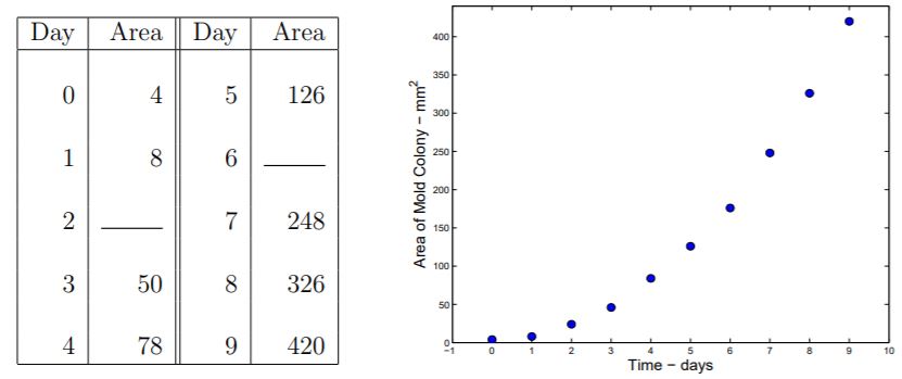
Figure \(\PageIndex{2}\): Areas of the mold colonies shown in Figure 1.5.1.

Explore 1.5.2 Do this. It is interesting and important to the remaining analysis. Find numbers A and B so that the graph of \(y=A l B^{t}\) approximates the mold growth data in Figure 1.5.1. Either chose two data points and insist that the points satisfy the equation or use a calculator or computer to compute the least squares approximation to the data. Similarly find a parabola \(y = a t^2 + b t + c\) that approximates the mold data. Draw graphs of the mold data, the exponential function, and the parabola that you found on a single set of axes.

Many people would expect the mold growth to be similar to bacterial growth and to have an exponential solution equation. We wish to explore the dynamics of mold growth.

Step 1. Mathematical model. Look carefully at the pictures in Figure 1.5.1. Observe that the features of the interior dark areas, once established, do not change. The growth is restricted to the perimeter of the colony⁷. On this basis we propose the model

Mathematical Model 1.5.1 Mold growth. Each day the increase in area of the colony is proportional to the length of the perimeter of the colony at the beginning of the day (when the photograph was taken).

Step 2. Notation. We will let \(t\) denote day of the experiment, \(A_t\) the area of the colony and \(C_t\) the length of the colony perimeter at the beginning of day \(t\).

Step 3. Dynamic equation. The statement that ‘a variable \(A\) is proportional to a variable \(B\)’ means that there is a constant, \(k\), and

\[A=k B\]

Thus, ‘the increase in area of the colony is proportional to the perimeter’ means that there is a constant, \(k\), such that

\[\text{ increase in area } =k \text{ perimeter }\]

The increase in the area of the colony on day \(t\) is \(A_{t+1} − A_{t}\), the area at the beginning of day \(t + 1\) minus the area at the beginning of day \(t\). We therefore write

\[A_{t+1}-A_{t}=k C_{t}\]

We now make the assumption that the mold colony is circular, so that⁸

\[C_{t}=2 \sqrt{\pi} \sqrt{A_{t}}\]

Therefore

\[A_{t+1}-A_{t}=k \cdot 2 \sqrt{\pi} \sqrt{A_{t}} \label{1.18}\]

Step 5. Solve the dynamic equation. The dynamic equation \ref{1.18} is difficult to solve, and may not have a useful formula for its solution⁹. The formula, \(A_{t} = 0\), defines a solution that is not useful. (Exercise 1.5.2).

A similar dynamic equation

\[A_{t+1}-A_{t-1}=K \sqrt{A_{t}} \label{1.19}\]

has a solution

\[A_{t}=\frac{K^{2}}{16} t^{2} \label{1.20}\]

and we ask you to confirm this solution in Exercise 1.5.5. The solution \(A_{t}=\frac{K^{2}}{16} t^{2}\) has \(A_{0} = 0\), which is not entirely satisfactory. (There was no mold on day 0.)

You are asked in Exercise 1.5.4 to estimate \(k \cdot 2 \sqrt{\pi}\) of Equation \ref{1.18} and to iteratively compute approximations to \(A_{0}, \cdots A_{9}\).

The difficulties at this stage lead us to reconsider the original problem.

Step 4. Reformulate the mathematical model. We have assumed the mold colony to be a circle expanding at its edges. We suggest that the radius is increasing at a constant rate, and write the following model.

Step 1. Mold growth, reformulated. Each day the radius of the colony increases by a constant amount.

Step 2. Notation, again. Let \(\rho _t\) be the radius¹⁰ of the colony at the beginning of day \(t\), and let \(\Delta\) (Greek letter delta) denote constant daily increase in radius.

Step 3. Dynamic equation, again. The increase in radius on day t is \(\rho _{t+1} − \rho _t\), the radius at the beginning of day \(t + 1\) minus the radius at the beginning of day \(t\), and we write

\[\rho_{t+1}-\rho_{t}=\Delta\]

Note

An important procedure in developing equations is to write a single thing two different ways, as we have just done for the increase in radius. Indeed, most equations do write a single thing two different ways.

You should check that the dimensions of the quantities on both sides of your equation are identical. This may assist in identifying dimensions of parameters in your equation.

Step 4. Solution equation, again. Convert \(\rho_{t+1}-\rho_{t}=\Delta\) to \[\rho_{t+1}=\rho_{t}+\Delta\] and write

\[\begin{aligned}
\rho_{1} &=\rho_{0}+\Delta \\
\rho_{2} &=\rho_{1}+\Delta \\
&=\left(\rho_{0}+\Delta\right)+\Delta \quad=\quad \rho_{0}+2 \Delta
\end{aligned}\]

and correctly guess that

\[\rho_{t}=\rho_{0}+t \Delta \label{1.22}\]

Evaluate \(\rho _0\) and \(\Delta\). From \(A_{t}=\pi \rho_{t}^{2}, \rho_{t}=\sqrt{A_{t} / \pi}\), and

\[\begin{array}{l}
\rho_{0}=\sqrt{A_{0} / \pi}=\sqrt{4 / \pi}=1.13 \\
\rho_{9}=\sqrt{A_{9} / \pi}=\sqrt{420 / \pi}=11.56
\end{array}\]

There are 9 intervening days between measurements \(\rho _0\) and \(\rho _9\) so the average daily increase in radius is

\[\Delta=\frac{11.56-1.13}{9}=1.16\]

We therefore write (\(\rho _{0} = 1.13, \Delta = 1.16\))

\[\rho_{t}=1.13+t 1.16\]

Now from \(A_{t}=\pi \rho_{t}^{2}\) we write

\[A_{t}=\pi(1.13+1.16 t)^{2} \label{1.23}\]

Step 6. Compare predictions from the model with observed data. A graph of \(A_{t}=\pi(1.13+1.16 t)^{2}\) and the original mold areas is shown in Figure 1.5.3 where we can see a reasonable fit, but there is a particularly close match at the two end points. It may be observed that only those two data points enter into calculations of the parameters 1.13 and 1.16 of the solution, which explains why the curve is close to them.

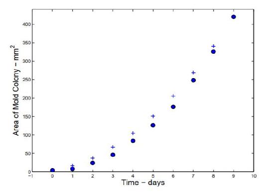
Figure \(\PageIndex{3}\): Comparison of the solution equation \ref{1.23} with the actual mold growth data.

Exercises for Section 1.5, Quadratic solution equations: Mold growth.

Exercise 1.5.1 You will have found in Explore 1.5.2 that the data is approximated pretty well by both an exponential function and a quadratic function. Why might you prefer a quadratic function?

Exercise 1.5.2 Show that \(A_{t} = 0\) for all \(t\) is a solution to Equation \ref{1.18},

\[A_{t+1}-A_{t}=2 \pi k \sqrt{A_{t}}\]

This means that for every \(t\), if \(A_{t} = 0\) and \(A_{t+1}\) is computed from the equation, then \(A_{t+1} = 0\) (and, yes, this is simple).

Exercise 1.5.3 Use data at days 2 and 8, (2, 24) and (8, 326), to evaluate \(\Delta\) and \(\rho _0\) in Equation \ref{1.22}

\[\rho_{t}=\rho_{0}+t \Delta\]

See Step 4, Solution Equation, Again.

Use the new values of \(\rho _0\) and \(\Delta\) in \(\rho_{t}=\rho_{0}+t \Delta\) to compute estimates of \(\rho_{0}, \rho_{1}, \cdots, \rho_{9}\) and \(A_{0}, A_{1}, \cdots, A_{9}\). Plot the new estimates of \(A_t\) and the observed values of \(A_t\) and compare your graph with Figure 1.5.3.

Exercise 1.5.4

1. Compute \(A_{t+1}-A_{t}\) and \(\sqrt{A_{t}}\) for the mold data in Figure 1.5.2 and plot \(A_{t+1}-A_{t} \text { vs } \sqrt{A_{t}}\). You should find that the line \(y = 5x\) lies close to the data. This suggests that 5 is the value of \(k \cdot 2 \sqrt{\pi}\) in Equation \ref{1.18}, \(A_{t+1}-A_{t}=k \cdot 2 \sqrt{\pi} \sqrt{A_{t}}\)
2. Use \[A_{0}=4, \quad A_{t+1}-A_{t}=5 \sqrt{A_{t}}\] to compute estimates of \(A_{1}, \cdots, A_{9}\). Compare the estimates with the observed data.
3. Find a value of \(K\) so that the estimates computed from \[A_{0}=4, \quad A_{t+1}-A_{t}=K \sqrt{A_{t}}\] more closely approximates the observed data than do the previous approximations.

Exercise 1.5.5 Examine the following model of mold growth:

Model of mold growth, III. The increase in area of the mold colony during any time interval is proportional to the length of the circumference of the colony at the midpoint of the time interval.

A schematic of a two-day time interval is

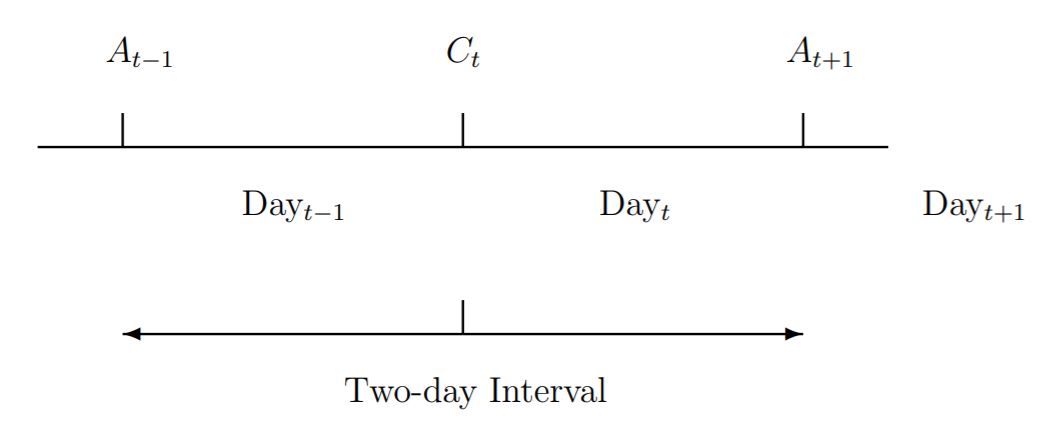
1. Explain the derivation of the dynamic equation \[A_{t+1}-A_{t-1}=k C_{t}\] from Model of mold growth, III. With \(C_{t}=2 \sqrt{\pi} \sqrt{A_{t}}=K \sqrt{A_{t}}\), the dynamic equation becomes \[A_{t+1}-A_{t-1}=K \sqrt{A_{t}}\]
2. Show by substitution that \[A_{t}=\frac{K^{2}}{16} t^{2} \quad \text { is a solution to } \quad A_{t+1}-A_{t-1}=K \sqrt{A_{t}}\] To do so, you will substitute \(A_{t+1}=\frac{K^{2}}{16}(t+1)^{2}, A_{t-1}=\frac{K^{2}}{16}(t-1)^{2}\), and \(A_{t}=\frac{K^{2}}{16} t^{2}\), and show that the left and right sides of the equation simplify to \(\frac{K^{2}}{4} t\).
3. When you find a value for \(K\), you will have a quadratic solution for mold growth. In the Figure 1.5.4 are values of \(A_{t+1}-A_{t-1}\) and \(\sqrt{A_{t}}\) and a plot of \(A_{t+1}-A_{t-1} \text { vs } \sqrt{A_{t}}\), with one data point omitted. Compute the missing data and identify the corresponding point on the graph.

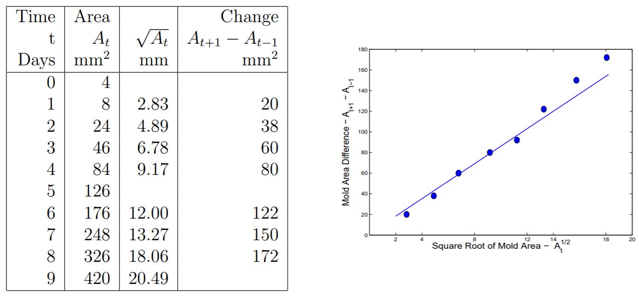
Figure \(\PageIndex{4}\): Data for Exercise 1.5.5, to estimate K in \(A_{t+1}-A_{t-1}=K \sqrt{A_{t}}\).

4. Also shown on the graph of \(A_{t+1} − A_{t−1} vs \sqrt{A_t}\) is the graph of \(y = 9.15 x\) which is the line of the form \(y = m x\) that is closest to the data. Let \(K = 9.15\) in \(A_{t} = \frac{K^2}{16} t^2\) and compute \(A_{0}, A_{1}, \cdots , A_{9}\). Compare the computed values with the observed values of mold areas.

Exercise 1.5.6 Suppose \(a, b\), and \(c\) are numbers and

\[P_{t}=a t^{2}+b t+c\]

where \(t\) is any number. Show that

\[Q_{t}=P_{t+1}-P_{t}\]

is linearly related to \(t\) (that is, \(Q_{t} = \alpha t + \beta\) for some \(\alpha\) and \(\beta\)), and that

\[R_{t}=Q_{t+1}-Q_{t}\]

is constant.

⁷ The pictures show the mold colony from above and we are implicitly taking the area of the colony as a measure of the colony size. There could be some cell division on the underside of the colony that would not be accounted for by the area. Such was not apparent from visual inspection during growth as a clear gelatinous layer developed on the underside of the colony.

⁸ For a circle of radius \(r\), \[\text { Area: } A=\pi r^{2}, \quad r=\sqrt{A / \pi}, \quad \text { Circumference: } \quad C=2 \pi r=2 \pi \sqrt{A / \pi}=2 \sqrt{\pi} \sqrt{A}\]

⁹ We spare you the details, but it can be shown that there is neither a quadratic nor exponential solution to Equation \ref{1.18}

¹⁰ We use the Greek letter \(\rho\) (rho) for the radius. We have already used \(R\) and \(r\) in another context.)