1.4: Doubling Time and Half-Life

Populations whose growth can be described by an exponential function (such as \(Pop = 0.022 (1.032)^T\)) have a characteristic doubling time, the time required for the population to double. The graph of the V. natriegens data and the graph of \(P = 0.022 (1.032)^T\) (Equation 1.1.5) that we derived from that data is shown in Figure 1.4.1. See Also: mathinsight.org/doubling_time_half_life_discrete

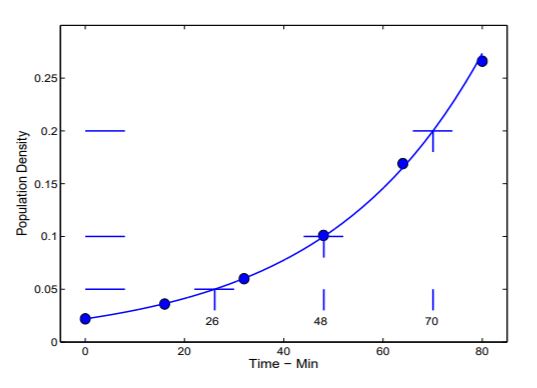
Figure \(\PageIndex{1}\): Data for V. natriegens growth and the graph of \(P = 0.022 (1.032)^T\).

Observe that at \(T = 26, P = 0.05\) and at \(T = 48, P = 0.1\); thus \(P\) doubled from 0.05 to 0.1 in the 22 minutes between \(T = 26\) and \(T = 48\). Also, at \(T = 70, P = 0.2\) so the population also doubled from 0.1 to 0.2 between \(T = 48\) and \(T = 70\), which is also 22 minutes.

The doubling time, \(T_{Double}\), can be computed as follows for exponential growth of the form

\[P=A B^{t} \quad B>1\]

Let \(P_1\) be the population at any time \(T_1\) and let \(T_2\) be the time at which the population is twice \(P_1\). The doubling time, \(T_{Double}\), is by definition \(T_{2} − T_{1}\) and

\[P_{1}=A B^{T_{1}} \quad \text { and } \quad P_{T_{2}}=2 P_{1}=A B^{T_{2}}\]

Therefore

\[\begin{align}
2 A B^{T_{1}} &=A B^{T_{2}} \\
2 &=\frac{B^{T_{2}}}{B^{T_{1}}} \\
2 &=B^{T_{2}-T_{1}} \\
T_{\mathrm{Double}}=T_{2}-T_{1} &=\frac{\log 2}{\log B} \quad \text { Doubling Time }
\end{align} \label{1.16}\]

Thus the doubling time for the equation \(P = A B^T\) is \(\log{2}/ \log{B}\). The doubling time depends only on \(B\) and not on \(A\) nor on the base of the logarithm. For the equation, \(Pop = 0.022 (1.032)^T\) , the doubling time is \(\log{2}/ \log{1.032} = 22.0056\), as shown in the graph.

Half Life

For the exponential equation \(y = A B^T\) with \(B < 1\), \(y\) does not grow. Instead, \(y\) decreases. The half-life, \(T_{Half}\), of \(y\) is the time it takes for \(y\) to one-half it initial size. The word, ‘half-life’ is also used in the context \(y = A B^x\) where \(x\) denotes distance instead of time. Data for light extinction below the surface of a lake from Section 1.3 on page 14 is shown in Figure 1.4.2 together with the graph of

\[I_{d}=0.4 (0.82)^{d}\]

Horizontal segments at \(Light = 0.4, Light = 0.2,\) and \(Light = 0.1\) cross the curve in Figure 1.4.2 at \(d = 0, d = 3.5\) and \(d = 7\). The ‘half-life’ of the light is 3.5 layers of water.

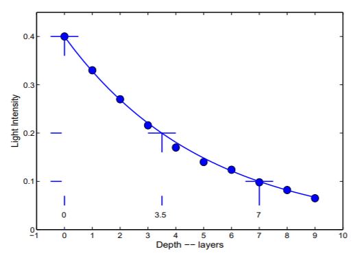
Figure \(\PageIndex{2}\): Graph of light intensity with depth and the curve \(I_{d} = 0.4 (0.82)^d\).

It might make more sense to you to call the number 3.5 the ‘half-depth’ of the light, but you will be understood by a wider audience if you call it ‘half-life’.

In Exercise 1.4.9 you are asked to prove that the half-life, \(T_{Half}\), of

\[\begin{align}
y=A B^{T}, & \text { where } B<1 \quad \text { is } \\
T_{\text {Half }}=\frac{\log \frac{1}{2}}{\log B} &=\frac{-\log 2}{\log B}
\end{align} \label{1.17}\]

Exercises for Section 1.4 Doubling Time and Half-Life.

Exercise 1.4.1 Determine the doubling times of the following exponential equations.

1. \(y = 2^t\)
2. \(y = 2^{3 t}\)
3. \(y = 2^{0.1 t}\)
4. \(y = 10^t\)
5. \(y = 10^{3 t}\)
6. \(y = 10^{0.1 t}\)

Exercise 1.4.2 Show that the doubling time of \(y=A B^{t}\) is \(1 /\left(\log _{2} B\right)\).

Exercise 1.4.3 Show that the doubling time of \(y=A (2)^{kt}\) is \(1 / k\).

Exercise 1.4.4 Determine the doubling times or half-lives of the following exponential equations.

1. \(y = 0.5^t\)
2. \(y = 2^{3 t}\)
3. \(y = 0.1^{0.1 t}\)
4. \(y = 100 (0.8)^t\)
5. \(y = 4 (5)^{3 t}\)
6. \(y = 0.0001 (5)^{0.1 t}\)
7. \(y = 10 (0.8)^{2 t}\)
8. \(y = 0.01 (3)^{t}\)
9. \(y = 0.01 ^{0.1 t}\)

Exercise 1.4.5 Find a formula for a population that grows exponentially and

1. Has an initial population of 50 and a doubling time of 10 years.
2. Has an initial population of 1000 and a doubling time of 50 years.
3. Has in initial population of 1000 and a doubling time of 100 years.

Exercise 1.4.6 An investment of amount \(A_0\) dollars that accumulates interest at a rate \(r\) compounded annually is worth

\[A_{t}=A_{0}(1+r)^{t}\]

dollars \(t\) years after the initial investment.

1. Find the value of \(A_{10}\) if \(A_{0} = 1\) and \(r = 0.06\).
2. For what value of \(r\) will \(A_{8} = 2\) if \(A_{0} = 1\)?
3. Investment advisers sometimes speak of the “Rule of 72”, which asserts that an investment at \(R\) percent interest will double in \(72/R\) years. Check the Rule of 72 for \(R = 4, R = 6, R = 8, R = 9,\) and \(R = 12\).

Exercise 1.4.7 Light intensities, \(I_1\) and \(I_2\), are measured at depths \(d\) in meters in two lakes on two different days and found to be approximately

\[I_{1}=2 (2)^{-0.1 d} \quad \text { and } \quad I_{2}=4 (2)^{-0.2 d}\]

1. What is the half-life of \(I_1\)?
2. What is the half-life of \(I_2\)?
3. Find a depth at which the two light intensities are the same.
4. Which of the two lakes is the muddiest?

Exercise 1.4.8

1. The mass of a single V. natriegens bacterial cell is approximately \(2 \cdot 10^{−11}\) grams. If at time 0 there are \(10^8\) V. natriegens cells in your culture, what is the mass of bacteria in your culture at time 0?
2. We found the doubling time for V. natriegen to be 22 minutes. Assume for simplicity that the doubling time is 30 minutes and that the bacteria continue to divide at the same rate. How many minutes will it take to have a mass of bacteria from Part a. equal one gram?
3. The earth weighs \(6 \cdot 10^{27}\) grams. How many minutes will it take to have a mass of bacteria equal to the mass of the Earth? How many hours is this? Why aren’t we worried about this in the laboratory? Why hasn’t this happened already in nature? Explain why it is not a good idea to extrapolate results far beyond the end-point of data gathering.

Exercise 1.4.9 Show that \(y = A (B)^t\) with \(B < 1\) has a half-life of

\[T_{\text {Half }}=\frac{\log \frac{1}{2}}{\log B}=\frac{-\log 2}{\log B}\]