1.1: Experimental data, bacterial growth.

Population growth was historically one of the first concepts to be explored in mathematical biology and it continues to be of central importance. Thomas Malthus in 1821 asserted a theory

“that human population tends to increase at a faster rate than its means of subsistence and that unless it is checked by moral restraint or disaster (as disease, famine, or war) widespread poverty and degradation inevitably result.” ²

In doing so he was following the bold arrows in Figure 1.1. World population has increased approximately six fold since Malthus’ dire warning, and adjustments using the additional network of the chart are still being argued.

Note

Duane Nykamp of the University of Minnesota is writing Math Insight, mathinsight.org, a collection of web pages and applets designed to shed light on concepts underlying a few topics in mathematics. One of the pages, mathinsight.org/bacterial_growth_initial_model, is an excellent display of the material of this section.

Bacterial growth data from a V. natriegens experiment are shown in Table 1.1. The population was grown in a commonly used nutrient growth medium, but the pH of the medium was adjusted to be pH 6.25 ³.

Table 1.1: Measurements of bacterial density. The units of “Population Density” are those of absorbance as measured by the spectrophotometer.

pH 6.25
Time (min)	Time Index \(t\)	Population Density \(B_t\)	Pop Change/Unit Time \((B_{t+1} − B_{t}) / 1\)
0	0	0.022	0.014
16	1	0.036	0.024
32	2	0.060	0.041
48	3	0.101	0.068
64	4	0.169	0.097
80	5	0.266

How do you measure bacteria density? Ideally you would place, say 1 microliter, of growth medium under a microscope slide and count the bacteria in it. This is difficult, so the procedure commonly used is to pass a beam of light through a sample of growth medium and measure the amount of light absorbed. The greater the bacterial density the more light that is absorbed and thus bacterial density is measured in terms of absorbance units. The instrument used to do this is called a spectrophotometer.

The spectrophotometer gives you a measure of light absorbance which is directly proportional to the bacterial density (that is, light absorbance is a constant times bacterial density). Absorbance is actually defined by

\[\text { Absorbance } \quad=\quad-\log _{10} \frac{I_{t}}{I_{0}}\]

where \(I_0\) is the light intensity passing through the medium with no bacteria present and It is the light intensity passing through the medium with bacteria at time \(t\). It may seem more natural to use

\[\frac{I_{0}-I_{t}}{I_{0}}\]

as a measure of absorbance. The reason for using \(log_{10} \frac{I_t}{I_0}\) is related to our next example for light absorbance below the surface of a lake, but is only easy to explain after continuous models are studied. See Chapter ?? (Exercise ??).

1.1.1 Steps towards building a mathematical model.

This section illustrates one possible sequence of steps leading to a mathematical model of bacterial growth.

Step 1. Preliminary Mathematical Model: Description of bacterial growth. Bacterial populations increase rapidly when grown at low bacterial densities in abundant nutrient. The population increase is due to binary fission – single cells divide asexually into two cells, subsequently the two cells divide to form four cells, and so on. The time required for a cell to mature and divide is approximately the same for any two cells.

Step 2. Notation. The first step towards building equations for a mathematical model is an introduction of notation. In this case the data involve time and bacterial density, and it is easy to let \(t\) denote time and \(B_t\) denote bacterial density at time t. However, the data was read in multiples of 16 minutes, and it will help our notation to rescale time so that \(t\) is 0, 1, 2, 3, 4, or 5. Thus B3 is the bacterial density at time \(3 \times 16 = 48\) minutes. The rescaled time is shown under ‘Time Index’ in Table 1.1.

Step 3. Derive a dynamic equation. In some cases your mathematical model will be sufficiently explicit that you are able to write the dynamic equation directly from the model. For this development, we first look at supplemental computations and graphs of the data.

Step 3a. Computation of rates of change from the data. Table 1.1 contains a computed column, ‘Population Change per Unit Time’. In the Mathematical Model, the time for a cell to mature and divide is approximately constant, and the overall population change per unit time should provide useful information.

Explore 1.1.1 Do this. It is important. Suppose the time for a cell to mature and divide is τ minutes. What fraction of the cells should divide each minute?

Using our notation,

\[B_{0}=0.022, \quad B_{1}=0.036, \quad B_{2}=0.060, \quad \text { etc. }\]

and

\[B_{1}-B_{0}=0.014, \quad B_{2}-B_{1}=0.024, \quad \text { etc. }\]

Step 3b. Graphs of the Data. Another important step in modeling is to obtain a visual image of the data. Shown in Figure 1.1.1 are three graphs that illustrate bacterial growth. Bacterial Growth A is a plot of column 3 vs column 2, B is a plot of column 4 vs column 2, and C is a plot of column 4 vs column 3 from the Table 1.1.

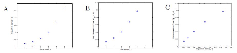
Figure \(\PageIndex{1}\): (A) Bacterial population density, \(B_t\) , vs time index, t. (B) Population density change per unit time, \(B_{t+1} − B_t\) , vs time index, \(t\). (C) Population density change per unit time, \(B_{t+1} − B_t\) , vs population density, \(B_t\) .

Note

In plotting data, the expression ‘plot B vs A’ means that B is the vertical coordinate and A is the horizontal coordinate. Students sometimes reverse the axes, and disrupt a commonly used convention that began some 350 years ago. In plotting bacterial density vs time, students may put bacterial density on the horizontal axis and time on the vertical axis, contrary to widely used practice. Perhaps if the mathematician who introduced analytic geometry, Rene DesCartes of France and Belgium, had lived in China where documents are read from top to bottom by columns and from right to left, plotting of data would follow another convention.

We suggest that you use the established convention.

The graph Bacterial Growth A is a classic picture of low density growth with the graph curving upward indicating an increasing growth rate. Observe from Bacterial Growth B that the rate of growth (column 4, vertical scale) is increasing with time.

The graph Bacterial Growth C is an important graph for us, for it relates the bacterial increase to bacterial density, and bacterial increase is based on the cell division described in our mathematical model. Because the points lie approximately on a straight line it is easy to get an equation descriptive of this relation. Note: See Explore 1.1.1.

Step 3c. An Equation Descriptive of the Data. Shown in Figure 1.1.2 is a reproduction of the graph Bacterial Growth C in which the point (0.15, 0.1) is marked with an ‘+’ and a line is drawn through (0, 0) and (0.15, 0.1). The slope of the line is 2/3. The line is ‘fit by eye’ to the first four points. The line can be ‘fit’ more quantitatively, but it is not necessary to do so at this stage.

Explore 1.1.2 Do this.

1. Why should the line in Figure 1.1.2 pass through (0, 0)?
2. Suppose the slope of the line is 2/3. Estimate the time required for a cell to mature and divide.

The fifth point, which is \((B_{4}, B_{5} − B_{4}) = (0.169, 0.097)\) lies below the line. Because the line is so close to the first four points, there is a suggestion that during the fourth time period, the growth, \(B_{5} − B_{4} = 0.97\), is below expectation, or perhaps, \(B_{5} = 0.266\) is a measurement error and should be larger. These bacteria were actually grown and measured for 160 minutes and we will find in Volume II, Chapter 14 that the measured value \(B_{5} = 0.266\) is consistent with the remaining data. The bacterial growth is slowing down after \(t = 4\), or after 64 minutes.

Figure \(\PageIndex{2}\): A line fit to the first four data points of bacterial growth. The line contains (0,0) and (0.15, 0.1) and has slope = 2/3.

The slope of the line in Bacterial Growth C is \(\frac{0.1}{0.15}=\frac{2}{3}\) and the y-intercept is 0. Therefore an equation of the line is

\[y=\frac{2}{3} x\]

Step 3d. Convert data equation to a dynamic equation. The points in Bacterial Growth C were plotted by letting \(x = B_t\) and \(y = B_{t+1} − B_{t}\) for \(t\) = 0, 1, 2, 3, and 4. If we substitute for x and y into the data equation \(y = \frac{2}{3} x\) we get \[B_{t+1}-B_{t}=\frac{2}{3} B_{t} \label{1.1}\] Equation \ref{1.1} is our first instance of a dynamic equation descriptive of a biological process.

Step 4. Enhance the preliminary mathematical model of Step 1. The preliminary mathematical model in Step 1 describes microscopic cell division and can be expanded to describe the macroscopic cell density that was observed in the experiment. One might extrapolate from the original statement, but the observed data guides the development.

In words Equation \ref{1.1} says that the growth during the \(t^{th}\) time interval is \(\frac{2}{3}\) times \(B_t\) , the bacteria present at time \(t\), the beginning of the period. The number \(\frac{2}{3}\) is called the relative growth rate - the growth per time interval is two-thirds of the current population size. More generally, one may say:

Mathematical Model 1.1.1 Bacterial Growth. A fixed fraction of cells divide every time period. (In this instance, two-thirds of the cells divide every 16 minutes.)

Step 5. Compute a solution to the dynamic equation. We first compute estimates of \(B_1\) and \(B_2\) predicted by the dynamic equation. The dynamic equation \ref{1.1} specifies the change in bacterial density \((B_{t+1} − B_{t})\) from \(t\) to time \(t + 1\). In order to be useful, an initial value of \(B_0\) is required. We assume the original data point, \(B_0 = 0.022\) as our reference point. It will be convenient to change \(B_{t+1} − B_{t} = \frac{2}{3} B_t\) into what we call an iteration equation:

\[B_{t+1}-B_{t}=\frac{2}{3} B_{t} \quad B_{t+1}=\frac{5}{3} B_{t} \label{1.2}\]

Iteration Equation \ref{1.2} is shorthand for at least five equations

\[B_{1}=\frac{5}{3} B_{0}, \quad B_{2}=\frac{5}{3} B_{1}, \quad B_{3}=\frac{5}{3} B_{2}, \quad B_{4}=\frac{5}{3} B_{3}, \quad \text { and } \quad B_{5}=\frac{5}{3} B_{4}\]

Beginning with \(B_{0} = 0.022\) we can compute

\[\begin{array}{l}
B_{1}=\frac{5}{3} B_{0}=\frac{5}{3} 0.022=0.037 \\
B_{2}=\frac{5}{3} B_{1}=\frac{5}{3} 0.037=0.061
\end{array}\]

Explore 1.1.3 Use \(B_{0} = 0.022\) and \(B_{t+1} = \frac{5}{3} B_t\) to compute \(B_{1}, B_{2}, B_{3}, B_{4}\), and \(B_{5}\). There is also some important notation used to describe the values of \(B_t\) determined by the iteration \(B_{t+1}=\frac{5}{3} B_{t}\). We can write

\[\begin{array}{lll}
B_{1} & =\frac{5}{3} B_{0} \\
B_{2} & =\frac{5}{3} B_{1} & B_{2}=\frac{5}{3}\left(\frac{5}{3} B_{0}\right) & =\frac{5}{3} \frac{5}{3} B_{0} \\
B_{3} & =\frac{5}{3} B_{2} & B_{3}=\frac{5}{3}\left(\frac{5}{3} \frac{5}{3} B_{0}\right) & =\frac{5}{3} \frac{5}{3} \frac{5}{3} B_{0}
\end{array}\]

Explore 1.1.4 Write an equation for B4 in terms of B0, using the pattern of the last equations.

At time interval 5, we get

\[B_{5}=\frac{5}{3} \frac{5}{3} \frac{5}{3} \frac{5}{3} \frac{5}{3} B_{0}\]

which is cumbersome and is usually written

\[B_{5}=\left(\frac{5}{3}\right)^{5} B_{0}\]

The general form is

\[B_{t}=\left(\frac{5}{3}\right)^{t} B_{0}=B_{0}\left(\frac{5}{3}\right)^{t} \label{1.3}\]

Using the starting population density, \(B_{0} = 0.022\), Equation \ref{1.3} becomes

\[B_{t}=0.022\left(\frac{5}{3}\right)^{t} \label{1.4}\]

and is the solution to the initial condition and dynamic equation \ref{1.1}

\[B_{0}=0.022, \quad B_{t+1}-B_{t}=\frac{2}{3} B_{t}\]

Populations whose growth is described by an equation of the form

\[P_{t}=P_{0} R^{t} \quad \text { with } \quad R>1\]

are said to exhibit exponential growth.

Equation \ref{1.4} is written in terms of the time index, \(t\). In terms of time, \(T\) in minutes, \(T = 16t\) and Equation \ref{1.4} may be written

\[B_{T}=0.022\left(\frac{5}{3}\right)^{T / 16}=0.022 (1.032)^{T} \label{1.5}\]

Step 6. Compare predictions from the Mathematical Model with the original data. How well did we do? That is, how well do the computed values of bacterial density, \(B_t\) , match the observed values? The original and computed values are shown in Figure 1.1.3.

pH 6.25
Time (min)	Time Index	Population Density	Computed Density
0	0	0.022	0.022
16	1	0.036	0.037
32	2	0.060	0.061
48	3	0.101	0.102
64	4	0.169	0.170
80	5	0.266	0.283

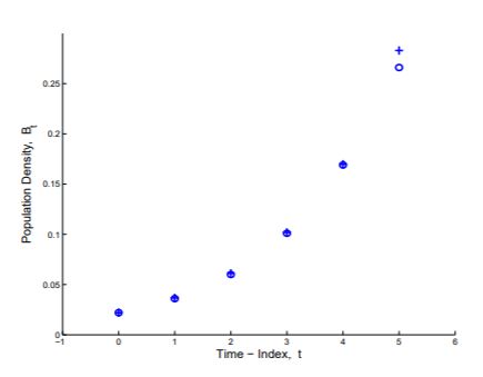
Figure \(\PageIndex{3}\): Tabular and graphical comparison of actual bacterial densities (o) with bacterial densities computed from Equation 1.3 (+).

The computed values match the observed values closely except for the last measurement where the observed value is less than the value predicted from the mathematical model. The effect of cell crowding or environmental contamination or age of cells is beginning to appear after an hour of the experiment and the model does not take this into account. We will return to this population with data for the next 80 minutes of growth in Section 15.6.1 and will develop a new model that will account for decreasing rate of growth as the population size increases.

1.1.2 Concerning the validity of a model.

We have used the population model once and found that it matches the data rather well. The validity of a model, however, is only established after multiple uses in many laboratories and critical examination of the forces and interactions that lead to the model equations. Models evolve as knowledge accumulates. Mankind’s model of the universe has evolved from the belief that Earth is the center of the universe, to the Copernican model that the sun is the center of the universe, to the realization that the sun is but a single star among some 200 billion in a galaxy, to the surprisingly recent realization (Hubble, 1923) that our Milky Way galaxy is but a single galaxy among an enormous universe of galaxies.

It is fortunate that our solution equation matched the data, but it must be acknowledged that two crucial parameters, \(P_0\) and \(r\), were computed from the data, so that a fit may not be a great surprise. Other equations also match the data. The parabola, \(y = 0.0236 + 0.000186 t + 0.00893 t^2\), computed by least squares fit to the first five data points is shown in Figure 1.1.4, and it matches the data as well as does \(P_{t} = 0.022(5/3)t\). We prefer \(P_{t} = 0.022(5/3)t\) as an explanation of the data over the parabola obtained by the method of least squares because it is derived from an understanding of bacterial growth as described by the model whereas the parabolic equation is simply a match of equation to data.

Exercises for Section 1.1, Experimental data, bacterial growth

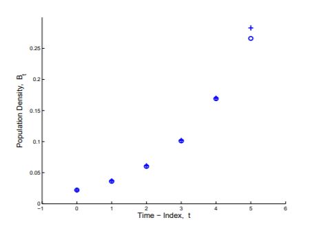
Figure \(\PageIndex{4}\): A graph of \(y=0.0236+.000186 t+0.00893 t^{2}\) (+) which is the quadratic fit by least squares to the first six data points (o) of V. natriegens growth in Table 1.1

Exercise 1.1.1 Compute B1, B2, and B3 as in Step 5 of this section for

1. \(B_{0}=4 \quad B_{t+1}-B_{t}=0.5 B_{t}\)
2. \(B_{0}=4 \quad B_{t+1}-B_{t}=0.1 B_{t}\)
3. \(B_{0}=0.2 \quad B_{t+1}-B_{t}=0.05 B_{t}\)
4. \(B_{0}=0.2 \quad B_{t+1}-B_{t}=1 B_{t}\)
5. \(B_{0}=100 \quad B_{t+1}-B_{t}=0.4 B_{t}\)
6. \(B_{0}=100 \quad B_{t+1}-B_{t}=0.01 B_{t}\)

Exercise 1.1.2 Write a solution equation for the initial conditions and dynamic equations of Exercise 1.1.1 similar to the solution Equation \ref{1.4}, \(B_{t} = (5/3)^{t}0.022\) of the pair \(B_{0} = 0.022, B_{t+1} − B_{t} = (2/3)B_{t} \).

Exercise 1.1.3 Observe that the graph Bacterial Growth C is a plot of \(B_{t+1} − B_{t} vs B_{t} \) The points are \(\left(B_{0}, B_{1}-B_{0}\right),\left(B_{1}, B_{2}-B_{1}\right)\), etc. The second coordinate, \(B_{t+1} − B_{t}\) is the population increase during time period \(t\), given that the population at the beginning of the time period is \(B_{t}\). Explain why the point (0, 0) would be a point of this graph.

Exercise 1.1.4 In Table 1.2 are given four sets of data. For each data set, find a number \(r\) so that the values \(B_{1}, B_{2}, B_{3}, B_{4}, B_{5}\) and \(B_6\) computed from the difference equation

\[B_{0}=\text { as given in the table, } \quad B_{t+1}-B_{t}=r B_{t}\]

are close to the corresponding numbers in the table. Compute the numbers, \(B_1\) to \(B_6\) using your value of \(r\) in the equation, \(B_{t+1} = (1 + r) B_t \), and compare your computed numbers with the original data.

For each data set, follow steps 3, 5, and 6. The line you draw close to the data in step 3 should go through (0, 0).

Exercise 1.1.5 The bacterium V. natriegens was also grown in a growth medium with pH of 7.85. Data for that experiment is shown in Table 1.3. Repeat the analysis in steps 1 - 9 of this section for this data. After completing the steps 1 - 9, compare your computed relative growth rate of V. natriegens at pH 7.85 with our computed relative growth rate of 2/3 at pH 6.25.

Exercise 1.1.6 What initial condition and dynamic equation would describe the growth of an Escherichia coli population in a nutrient medium that had 250,000 E. coli cells per milliliter at the start of an experiment and one-fourth of the cells divided every 30 minutes.

Table 1.2: Tables of data for Exercise 1.1.4

(a)		(b)		(c)		(d)
\(t\)	\(B_t\)	\(t\)	\(B_t\)	\(t\)	\(B_t\)	\(t\)	\(B_t\)
0	1.99	0	0.015	0	22.1	0	287
1	2.68	1	0.021	1	23.4	1	331
2	3.63	2	0.031	2	26.1	2	375
3	4.89	3	0.040	3	27.5	3	450
4	6.63	4	0.055	4	30.5	4	534
5	8.93	5	0.075	5	34.4	5	619
6	12.10	6	0.106	6	36.6	6	718

Table 1.3: Data for Exercise 1.1.5, V. natriegens growth in a medium with pH of 7.85.

pH 7.85
Time (min)	Population Density
0	0.028
16	0.047
32	0.082
48	0.141
64	0.240
80	0.381

² Merriam Webster’s Collegiate Dictionary, Tenth Edition.

³ The experiment was a semester project of Deb Christensen in which several V. natriegens populations were grown in a range of pH values.