1.3: Experimental data - Sunlight depletion below the surface of a lake or ocean

Light extinction with increasing depth of water determines underwater plant, algae, and phytoplankton growth and thus has important biological consequences. We develop and analyze a mathematical model of light extinction below the surface of the ocean.

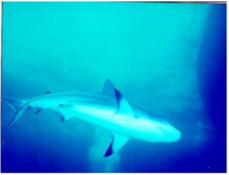
Figure \(\PageIndex{1}\): There is less light in the water below the shark than there is in the water above the shark.

Sunlight is the energy source of almost all life on Earth and its penetration into oceans and lakes largely determines the depths at which plant, algae and phytoplankton life can persist. This life is important to us: some 85% of all oxygen production on earth is by the phytoplankta diatoms and dinoflagellates⁴.

Explore 1.3.1 Preliminary analysis. Even in a very clear ocean, light decreases with depth below the surface, as illustrated in Figure 1.3.1. Think about how light would decrease if you were to descend into the ocean. Light that reaches you passes through the water column above you.

1. Suppose the light intensity at the ocean surface is \(I_0\) and at depth 10 meters the light intensity is \(\frac{1}{2} I_0\). What light intensity would you expect at 20 meters?
2. Draw a candidate graph of light intensity versus depth.

We are asking you to essentially follow the bold arrows of the chart in Figure 1.3.2.

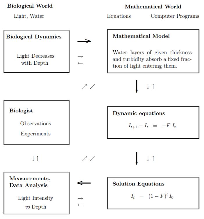
Figure \(\PageIndex{2}\): Biology - Mathematics: Information Flow Chart for the sunlight depletion example.

The steps in the analysis of light depletion are analogous to the steps for the analysis of bacterial growth in Section 1.1.

Step 1. Statement of a mathematical model. Think of the ocean as divided into layers, say one meter thick, as illustrated in Figure 1.8. As light travels downward from the surface, each layer will absorb some light. We will assume that the distribution of suspended particles in the water is uniform so that the light absorbing properties of each two layers are the same. We hypothesize that each two layers will absorb the same fraction of the light that enters it. The magnitude of the light absorbed will be greater in the top layers than in the lower layers simply because the intensity of the light entering the the top layers is greater than the intensity of light at the lower layers. We state the hypothesis as a mathematical model.

Mathematical Model 1.3.1 Light depletion with depth of water. Each layer absorbs a fraction of the light entering the layer from above. The fraction of light absorbed, f, is the same for all layers of a fixed thickness.

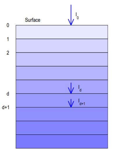
Figure \(\PageIndex{3}\): A model of the ocean partitioned into layers.

Step 2. Notation. We will let \(d\) denote depth (an index measured in layers) and \(I_d\) denote light intensity at depth \(d\). Sunlight is partly reflected by the surface, and \(I_0\) (light intensity at depth 0) is to be the intensity of the light that penetrates the surface. \(I_1\) is the light intensity at the bottom of the first layer, and at the top of the second layer.

The opacity⁵ of the water is due generally to suspended particles and is a measure of the turbidity of the water. In relatively clear ocean water, atomic interaction with light is largely responsible for light decay. In the bacterial experiments, the growth of the bacteria increases the turbidity of the growth serum, thus increasing the opacity and the absorbance.

The fraction, \(f\), of light absorbed by each layer is between 0 and 1 (or possibly 1, which would not be a very interesting model). Although \(f\) is assumed to be the same for all layers, the value of \(f\) depends on the thickness of the layer and the distribution of suspended particles in the water and atomic interactions with light. Approximately,

\[f= \text{ Layer thickness } \times \text{ Opacity of the water }\].

Layer thickness should be sufficiently thin that the preceding approximation yields a value of \(f\) substantially less than 1. We are developing a discrete model of continuous process, and need layers thin enough to give a good approximation. The continuous model is shown in Subsection 5.5.2. Thus for high opacity of a muddy lake, layer thickness of 20 cm might be required, but for a sparkling ocean, layer thickness of 10 m might be acceptable.

Explore 1.3.2 Assume that at the surface light intensity I0 is 400 watts/meter-squared and that each layer of thickness 2 meters absorbs 10% of the light that enters it. Calculate the light intensity at depths 2, 4, 6, · · ·, 20 meters. Plot your data and compare your graph with the graph you drew in Explore 1.3.1.

Step 3. Develop a dynamic equation representative of the model. Consider the layer between depths \(d\) and \(d + 1\) in Figure 1.3.3. The intensity of the light entering the layer is \(I_d\).

Note

The light absorbed by the layer between depths \(d\) and \(d + 1\) is the difference between the light entering the layer at depth d and the light leaving the layer at depth \(d + 1\), which is \(I_{d} − I_{d+1}\).

The mathematical model asserts that

\[I_{d}-I_{d+1}=f I_{d} \label{1.10}\]

Note that \(I_d\) decreases as \(d\) increases so that both sides of Equation \ref{1.10} are positive. It is more common to write

\[I_{d+1}-I_{d}=-f I_{d} \label{1.11}\]

and to put this equation in iteration form

\[I_{d+1}=(1-f) I_{d} \quad I_{d+1}=F I_{d} \label{1.12}\]

where \(F = 1 − f\). Because \(0 < f < 1\), also \(0 < F < 1\).

Step 4. Enhance the mathematical model of Step 1. We are satisfied with the model of Step 1 (have not yet looked at any real data!), and do not need to make an adjustment.

Step 5. Solve the dynamical equation, \(I_{d+1} − I_{d} = −f I_{d}\). The iteration form of the dynamical equation is \(I_{d+1} = F I_d\) and is similar to the iteration equation \(B_{t+1} = \frac{5}{3} B_t\) of bacterial growth for which the solution is \(B_{t}=B_{0}\left(\frac{5}{3}\right)^{t}\). We conclude that the solution of the light equation is

\[I_{d}=I_{0} F^{d} \label{1.13}\]

The solutions,

\[B_{t}=B_{0}\left(\frac{5}{3}\right)^{t} \quad \text{and} \quad I_{d}=I_{0} F^{d} \quad F<1\]

are quite different in character, however, because \(\frac{5}{3} > 1, (\frac{5}{3})^t\) increases with increasing \(t\) and for \(F < 1, F^d\) decreases with increasing \(d\).

Step 6. Compare predictions from the model with experimental data. It is time we looked at some data. We present some data, estimate f of the model from the data, and compare values computed from Equation \ref{1.13} with observed data.

In measuring light extinction, it is easier to bring the water into a laboratory than to make measurements in a lake, and our students have done that. Students collected water from a campus lake with substantial suspended particulate matter (that is, yucky). A vertically oriented 3 foot section of 1.5 inch diameter PVC pipe was blocked at the bottom end with a clear plastic plate and a flashlight was shined into the top of the tube (see Figure 1.3.4). A light detector was placed below the clear plastic at the bottom of the tube. Repeatedly, \(30 cm^3\) of lake water was inserted into the tube and the light intensity at the bottom of the tube was measured. One such data set is given in Figure 1.9 ⁶.

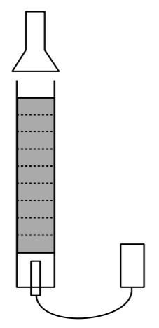
Depth Layer	\(I_{d} \quad mW/cm^2\)	\(I_{d+1} - I_{d} \quad mW/cm^2\)
0	0.400	-0.070
1	0.330	-0.060
2	0.270	-0.054
3	0.216	-0.046
4	0.170	-0.030
5	0.140	-0.016
6	0.124	-0.026
7	0.098	-0.016
8	0.082	-0.017
9	0.065

Figure \(\PageIndex{4}\): Diagram of laboratory equipment and data obtained from a light decay experiment.

Explore 1.3.3 In Figure 1.3.5A is a graph of \(I_d\) vs \(d\). Compare this graph with the two that you drew in Explore 1.3.1 and 1.3.2.

Our dynamical equation relates \(I_{d+1} − I_d\) to \(I_d\) and we compute change in intensity, \(I_{d+1} − I_d\), just as we computed changes in bacterial population. The change in intensity, \(I_{d+1} − I_d\), is the amount of light absorbed by layer, \(d\).

Graphs of the data. A graph of the original data, \(I_d\) vs \(d\), is shown in Figure 1.3.5(A) and and a graph of \(I_{d+1} − I_d\) vs \(I_d\) is shown in Figure 1.3.5(B).

In Figure 1.3.5(B) we have drawn a line close to the data that passes through (0,0). Our reason that the line should contain (0,0) is that if \(I_d\), the amount of light entering layer d is small, then \(I_{d+1} − I_d\), the amount of light absorbed by that layer is also small. Therefore, for additional layers, the data will cluster near (0,0).

The graph of \(I_{d+1} − I_d\) vs \(I_d\) is a scattered in its upper portion, corresponding to low light intensities. There are two reasons for this.

1. Maintaining a constant light source during the experiment is difficult so that there is some error in the data.

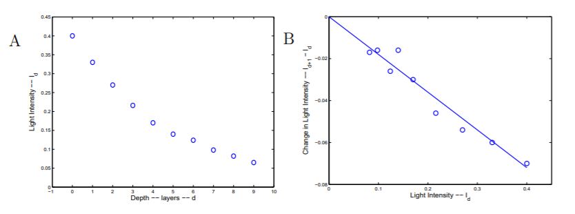
Figure \(\PageIndex{5}\): (A) The light decay curve for the data of Figure 1.3.4 and (B) the graph of light absorbed by layers vs light entering the layer from Table 1.3.4.

2. Subtraction of numbers that are almost equal emphasizes the error, and in some cases the error can be as large as the difference you wish to measure. In the lower depths, the light values are all small and therefore nearly equal so that the error in the differences is a large percentage of the computed differences.

Use the data to develop a dynamic equation. The line goes through (0,0) and the point (0.4, -0.072). An equation of the line is

\[y=-0.18 x\]

Remember that \(y\) is \(I_{d+1} − I_d\) and \(x\) is \(I_d\) and substitute to get

\[I_{d+1}-I_{d}=-0.18 I_{d}\]

This is the dynamic Equation \ref{1.11} with \(−f = −0.18\).

Solve the dynamic equation. (Step 5 for this data.) The iteration form of the dynamic equation is

\[I_{d+1}=I_{d}-0.18 I_{d} \quad I_{d+1}=0.82 I_{d}\]

and the solution is (with \(I_{0} = 0.400\))

\[I_{d}=0.82^{d} \quad I_{0}=0.4000 ~ .82^{d} \label{1.15}\]

Compare predictions from the Mathematical Model with the original data. How well did we do? Again we use the equations of the model to compute values and compare them with the original data. Shown in Figure 1.3.6 are the original data and data computed with \(\hat{I}_{d}=0.400 (0 .82)^{d}\), and a graph comparing them.

The computed data match the observed data quite well, despite the ‘fuzziness’ of the graph in Figure 1.3.5(b) of \(I_{d+1}-I_{d} \text { vs } I_{d}\) from which the dynamic equation was obtained.

Depth Layer	\(I_d\) Observed	\(\hat{I}_{d}\) Computed
0	0.400	0.400
1	0.330	0.328
2	0.270	0.269
3	0.216	0.221
4	0.170	0.181
5	0.140	0.148
6	0.124	0.122
7	0.098	0.100
8	0.082	0.082
9	0.065	0.067

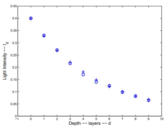
Figure \(\PageIndex{6}\): Comparison of original light intensities (o) with those computed from \(\hat{I}_{d}=0.82^{d} 0.400\) (+).

Exercises for Section 1.3, Experimental data: Sunlight depletion below the surface of a lake or ocean.

Exercise 1.3.1 In Table 1.4 are given four sets of data that mimic light decay with depth. For each data set, find a number \(r\) so that the values \(B_{1}, B_{2}, B_{3}, B_{4}, B_{5}\) and \(B_{6}\) computed from the difference equation

\[B_{0}=\text { as given in the table, } \quad B_{t+1}-B_{t}=-r B_{t}\]

are close to the corresponding numbers in the table. Compute the numbers, \(B_1\) to \(B_6\) using your value of \(R\) in the equation and compare your computed numbers with the original data.

For each data set, follow steps 3, 5, and 6. The line you draw close to the data in step 3 should go through (0,0).

Table 1.4: Tables of data for Exercise 1.3.1

(a)		(b)		(c)		(d)
\(t\)	\(B_t\)	\(t\)	\(B_t\)	\(t\)	\(B_t\)	\(t\)	\(B_t\)
0	3.01	0	20.0	0	521	0	0.85
1	2.55	1	10.9	1	317	1	0.65
2	2.14	2	5.7	2	189	2	0.51
3	1.82	3	3.1	3	119	3	0.40
4	1.48	4	1.7	4	75	4	0.32
5	1.22	5	0.9	5	45	5	0.25
6	1.03	6	0.5	6	28	6	0.19

Exercise 1.3.2 Now it is your turn. Shown in the Exercise Table 1.3.2 are data from a light experiment using the laboratory procedure of this section. The only difference is the water that was used. Plot the data, compute differences and obtain a dynamic equation from the plot of differences vs intensities. Solve the dynamic equation and compute estimated values from the intensities and compare them with the observed light intensities. Finally, decide whether the water from your experiment is more clear or less clear than the water in Figure 1.3.4. (Note: Layer thickness was the same in both experiments.)

Table for Exercise 1.3.2 Data for Exercise 1.3.2.

Depth Layer	0	1	2	3	4	5	6	7	8
Light Intensity	0.842	0.639	0.459	0.348	0.263	0.202	0.154	0.114	0.085

Exercise 1.3.3 One might reasonably conclude that the graph in Figure 1.3.5(a) looks like a parabola. Find an equation of a parabola close to the graph in Figure 1.3.5(a). Your calculator may have a program that fits quadratic functions to data, or you may run the MATLAB program:

Code \(\PageIndex{1}\) (MATLAB):

close all;clc;clear
D=[0:1:9];
I=[0.4 0.33 0.27 0.216 0.17 0.14 0.124 0.098 0.082 0.065];
P=polyfit(D,I,2)
X=[0:0.1:9]; Y=polyval(P,X);
plot(D,I,’o’,’linewidth’,2);
hold(’on’);
plot(X,Y,’linewidth’,2)

The structure of a program to fit a parabola to data is:

1. Close and clear all previous graphs and variables. [Perhaps unnecessary.]
2. Load the data. [In lists D (depths) and I (light intensity)].
3. Compute the coefficients of a second degree polynomial close to the data and store them in P.
4. Specify X coordinates for the polynomial and compute the corresponding Y coordinates of the polynomial.
5. Plot the original data as points.
6. Plot the computed polynomial.

Compare the fit of the parabola to the data in Figure 1.1.5(a) with the fit of the graph of \(I_{d}=0.400(0 .82)^{d}\) to the same data illustrated in Figure 1.1.6.

The parabola fits the data quite well. Why might you prefer \(I_{d}=0.400(0 .82)^{d}\) over the equation of the parabola as an explanation of the data?

Exercise 1.3.4 A light meter suitable for underwater photography was used to measure light intensity in the ocean at Roatan, Honduras. The meter was pointed horizontally. Film speed was set at 400 ASA and time at 1/60 s. The recommended shutter apertures (\(f\) stop) at indicated depths are shown in Table Ex. 1.3.4. We show below that the light intensity is proportional to the square of the recommended shutter aperture. Do the data show exponential decay of light?

Notes. The quanta of light required to expose the 400 ASA film is a constant, \(C\). The amount of light that strikes the film in one exposure is \(A \Delta T I\), where \(A\) is area of shutter opening, \(\Delta T\) is the time of exposure (set to be 1/60 s) and I is light intensity (quanta/(\(cm2 -sec\))). Therefore

\[ C=A \Delta T \times I \quad \text { or } \quad I=C \frac{1}{\Delta T} \frac{1}{A}=60 C \frac{1}{A}\]

By definition of \(f\)-stop, for a lense of focal length, \(F\), the diameter of the shutter opening is \(F\)/(\(f\)-stop) mm. Therefore

\[A=\pi\left(\frac{F}{f-\operatorname{stop}}\right)^{2}\]

The last two equations yield

\[I=60 C \frac{1}{\pi} \frac{1}{F^{2}}(f-\text { stop })^{2}=K(f-\text { stop })^{2} \quad \text { where } \quad K=60 C \frac{1}{\pi} \frac{1}{F^{2}}\]

Thus light intensity, \(I\) is proportional to \((f-\operatorname{stop})^{2}\).

Table for Exercise 1.3.4 \(f\)-stop specifications for 400 ASA film at 1/60 s exposure at various depths below the surface of the ocean near Roatan, Honduras.

Depth (m)	\(f\)-stop
3	16
6	11
9	8
12	5.6
15	4

⁴ PADI Diving Encyclopedia

⁵ Wikipedia. Opacity – the degree to which light is not allowed to travel through. Turbidity– the cloudiness or haziness of a fluid caused by individual particles (suspended particles) that are generally invisible to the naked eye.

⁶ This laboratory is described in Brian A. Keller, Shedding light on the subject, Mathematics Teacher 91 (1998), 756-771.