3.1: Tangent to the Graph of a Function

Elementary and very important.

Consider a line with equation,

\(y = m x + b\).

The slope, m, of the line is computed as the increment in y divided by the increment in x between two points of the line, and may be called the rate of change of y with respect to x.

• If y measures bacterial population size at time x measured in hours, the slope m is the bacterial increase per hour, or bacterial growth rate, with dimensions, pop/hour.
• If y measures the height of a young girl in inches at year x, then m is the growth rate of the girl in inches per year.
• If y measures a morphogen concentration a distance x from its source in a developing embryo, m is the rate of concentration decrease, called a morphogenetic gradient, that causes differentiation of specific cell types in a distinct spatial order.

The simple rate of change of linear functions is crucial to understanding the rate of change of nonlinear functions.

Example 3.1.1 At what rate was the Vibrio natriegens population of Section 1.1 growing at time T = 40 minutes?

We have data for population density (measured in absorbance units) at times T = 0, T = 16, T = 32, T = 48, T = 64, and T = 80, minutes.

Time	0	16	32	48	64	80
Absorbance	0.022	0.036	0.060	0.101	0.169	0.266

The average growth rate between times T = 32 and T = 48 is

\[\frac{0.101-0.060}{48-32}=0.0026 \quad \frac{\text { Absorbance units }}{\text { minute }}\]

and is a pretty good estimate of the growth rate at time T = 40, particularly because 40 is midway between 32 and 48.

In Section 1.1 we let t index time in 16 minutes intervals, and we used the mathematical model that population increase during time t to t + 1 is proportional to the population at time t. With \(B_t\) being population at time index t, we wrote

\[B_{t+1}-B_{t}=r \times B_{t} \quad \text { for } \quad t=0,1,2,3,4,5 \label{3.1}\]

We concluded that

\[B_{t}=0.022\left(\frac{5}{3}\right)^{t}, \quad \text { for } \quad t=0,1,2,3,4,5\]

In terms of T in minutes and B(T) in absorbance units, (Equation 1.1.5)

\[B(T)=0.022\left(\frac{5}{3}\right)^{T / 16}=0.022 \cdot 1.032^{T} \label{3.2}\]

Shown in Figure 3.1.1A are the data, the discrete computations of Equation \ref{3.1} and the graph of Equation \ref{3.2}. A magnification of the graph near T = 40 minutes is shown Figure 3.1.1B together with a tangent drawn at ( 40, B(40) ).

Figure \(\PageIndex{1}\): A. Graph of the V. natriegens data (+), the discrete approximation of Equation \ref{3.1} (filled circles) and the graph of Equation \ref{3.2}. A magnification near T = 40 minutes is shown in B together with a tangent to the graph of B(T) (Equation \ref{3.2}) at ( 40, B(40) ).

We define the (instantaneous) growth rate of a population described by B(T) at time T = 40 to be the slope of the tangent to the graph of B at time T = 40. The units on the slope of the tangent are

\[\frac{\text { change in } \mathrm{y}}{\text { change in } \mathrm{x}}=\frac{\text { Absorbance units }}{\text { Time in seconds }}\]

and are appropriate for population growth rate. Shown in Figure 3.1.2 are the tangent and a secant line between ( 32, B(32) ) and ( 48, B(48) ). The slope of the secant is

\[\frac{B(48)-B(32)}{48-32}=\frac{0.10185-0.06111}{16}=0.002546\]

This is the average growth rate of B and is slightly different from the average growth rate (0.0026) computed from the data because B only approximates the data (pretty well, actually) and can be computed with higher accuracy than is possible with the data.

We can compute a closer estimate of the slope of the tangent by computing

\[\frac{B(45)-B(35)}{45-35}=\frac{0.092549-0.067254}{10}=0.0025295\]

It would be possible to have absorbance data at 5 minute intervals and compute the average growth rate between 35 and 45 minutes, but there are two difficulties. The main difficulty is that absorbance (on our machine) can only be measured to three decimal digits and the answer could be trusted to only 3 decimal digits, the first of which is 0. A second problem is that at each reading, 10 ml of growth serum is extracted, analyzed in the spectrophotemeter, and discarded. In 80 minutes, 160 ml of serum would be discarded, possibly more than was initially present.

Figure \(\PageIndex{2}\): Graph of B(T), the tangent to the graph at ( 40, B(40) ) and the secant through ( 32, B(32) ) and ( 48, B(48) ).

Example 3.1.2 At what rate was the world human population increasing in 1980? Shown in Figure 3.1.3 are data for the twentieth century and a graph of an approximating function, F. A tangent to the graph of F at (1980, F(1980)) is drawn and has a slope of \(0.0781 \cdot 10^{9} = 78, 100, 000\). Now,

\[\text { slope is } \quad \frac{\text { rise }}{\text { run }}=\frac{\text { change in population }}{\text { change in years }} \approx \frac{\text { people }}{\text { year }}\]

The units of slope, then, are people/year. Therefore,

\[\text { slope }=78,100,000 \frac{\text { people }}{\text { year }}\]

The world population was increasing approximately 78,100,000 people per year in 1980.

Explore 3.1.1 At approximately what rate was the world human population increasing in 1920?

Definition 3.1.1 Rate of change of a function at a point.

If the graph of a function, F, has a tangent at a point (a, F(a)), then the rate of change of F at a is the slope of the tangent to F at the point (a, F(a)).

Figure \(\PageIndex{3}\): Graph of United Nations estimates of world human population for the twentieth century, an approximating curve, and a tangent to the curve. The slope of the tangent is \(0.0781 \cdot 10^{9} = 78, 100, 000.\)

Figure \(\PageIndex{4}\): In neither of these graphs will we accept a line as tangent to the graph at the point (2,3)

To be of use, Definition 3.1.1 requires a definition of tangent to a graph which is given below in Definition 3.1.3. In some cases there will be no tangent. In each graph shown in Figure 3.1.4 there is no tangent at the point (3,2) of the graph. Students usually agree that there is no tangent in graphs A and B, but sometimes argue about case C.

Explore 3.1.2 Do you agree that there is no line tangent to any of the graphs in Figure 3.1.4 at the point (3,2)?

Examples of tangents to graphs are shown in Figure 3.1.5; all the graphs have tangents at the point (2, 4). In Figure 3.1.5C, however, the line shown is not the tangent line. The graphs in B and C are the same and the tangent at (2, 4) is the line drawn in B.

A line tangent to the graph of \(F\) at a point \((a, F(a))\) contains (a, F(a)) so in order to find the tangent we only need to find the slope of the tangent, which we denote by \(m_a\). To find \(m_a\) we consider points \(b\) in the domain of \(F\) that are different from a and compute the slopes,

\[\frac{F(b)-F(a)}{b-a}\]

of the lines that contain \((a, F(a))\) and \((b, F(b))\). The line containing \((a, F(a))\) and \((b, F(b))\) is called a secant of the graph of \(F\). The slope, \(\frac{F(b) − F(a)}{b − a}\), of the secant is a ’good’ approximation to the slope of the tangent when b is ’close to’ a. A graph, a tangent to the graph, and a secant to the graph are shown in Figure 3.1.6. If we could animate that figure, we would slide the point \((b, F(b))\) along the curve towards \((a, F(a))\) and show the secant moving toward the tangent.

Figure \(\PageIndex{5}\): All of these graphs have a tangent to the graph at the point (2,4). However, the line drawn in C is not the tangent.

Figure \(\PageIndex{6}\): A graph, a tangent to the graph, and a secant to the graph.

A substitute for this animation is shown in Figure 3.1.7. Three points are shown, \(B_{1}, B_{2}\), and \(B_3\) with \(B_{1} = ( b_{1}, F(b_{1}) )\), \(B_{2} = ( b_{2}, F(b_{2}) )\), and \(B_{3} = ( b_{3}, F(b_{3}) )\). The numbers \(b_{1}, b_{2}\), and \(b_{3}\) are progressively closer to \(a\), and the slopes of the dashed lines from \(B_{1}, B_{2}\), and \(B_{3}\) to \((a,F(a))\) are progressively closer to the slope of the tangent to the graph of \(F\) at \((a, F(a))\). Next look at the magnification of \(F\) in Figure 3.1.7B. The progression toward a continues with \(b_{3}, b_{4}\), and \(b_{5}\), and the slopes from \(B_{3}, B_{4}\), and \(B_{5}\) to \((a, F(a))\) move even closer to the slope of the tangent.

Explore 3.1.3 It is important in Figure 3.1.7 that as the x-coordinates \(b_{1}, b_{2}, \cdots\) approach a the points \(B_{1} = ( b_{1}, F(b_{1}) ), B_{2} = ( b_{2}, F(b_{2}) ), \cdots\) on the curve approach \((a, f(a))\). Would this be true in Figure 3.1.4B?

Figure \(\PageIndex{7}\): A. A graph and tangent to the graph at \((a, F(a))\). Slopes of the secant lines from \(B_{1}, B_{2},\) and \(B_3\) to \((a, F(a))\) progressively move toward the slope of the tangent. B. A magnification of A with the progression continued.

Definition 3.1.2

Suppose \(a\) and \(b\) are two numbers and \(a < b\). The open interval, \((a, b)\) consists of all of the numbers between \(a\) and \(b\) (not including either \(a\) or \(b\)). The closed interval, \([a, b]\) consists of \(a\), all of the numbers between \(a\) and \(b\), and \(b\).

The notation for open interval is ambiguous. (3,5) might represent all the numbers between 3 and 5 or might represent the point in the plane whose coordinate pair is (3,5). The context of it use should clarify its meaning.

Definition 3.1.3

Suppose the domain of a function \(F\) contains an open interval that contains a number \(a\). Suppose further that there is a number \(m_a\) such that that for points \(b\) in the interval different from \(a\),

\[\text{as } b \text{ approaches } a \quad \frac{F(b)-F(a)}{b-a} \quad \text{approaches } m_a\]

Then \(m_a\) is the slope of the tangent to \(F\) at \((a, F(a))\). The graph of \(y = F(a) + m_{a}(x − a)\) is the tangent to the graph of \(F\) at \((a, F(a))\).

We are making progress. We now have a definition of tangent to a graph and therefore have given meaning to rate of change of a function. However, we must make sense of the phrase

\[\text{as } b \text{ approaches } a \quad \frac{F(b)-F(a)}{b-a} \quad \text{approaches } m_a\]

This phrase is a bridge between geometry and analytical computation and is formally defined in Definition 3.2.1. We first use it on an intuitive basis. Some students prefer an alternate, similarly intuitive statement:

\[\text { if } b \text { is close to } a \quad \frac{F(b)-F(a)}{b-a} \quad \text { is close to } m_{a}\]

Both phrases are helpful.

Consider the parabola, shown in Figure 3.1.8,

\[F(t)=t^{2} \quad \text { for all } t \text { and a point }\left(a, a^{2}\right) \text { of } F\]

Figure \(\PageIndex{8}\): The parabola, \(F(t) = t^2\), a tangent to the parabola at \((a, a^{2} )\), and a secant through \((a, a^{2} )\) and \((b, b^{2} )\).

The slope of the secant is

\[\frac{F(b)-F(a)}{b-a}=\frac{b^{2}-a^{2}}{b-a}=\frac{(b-a)(b+a)}{b-a}=b+a\]

Although 'approaches’ has not been carefully defined, it should not surprise you if we conclude that

\[\text{ as } b \text { approaches } a \quad \frac{F(b)-F(a)}{b-a}=\frac{b^{2}-a^{2}}{b-a}=b+a \quad \text { approaches } \quad a+a=2 a .\]

Alternatively, we might conclude that

\[\[\text{ if } b \text { is close to } a \quad \frac{F(b)-F(a)}{b-a}=\frac{b^{2}-a^{2}}{b-a}=b+a \quad \text { is close to } \quad a+a=2 a .\]

We make either conclusion, and along with it conclude that the slope of the tangent to the parabola \(y = x^2\) at the point \((a, a^{2})\) is \(2a\). Furthermore, the rate of change of \(F(t) = t^2\) at \(a\) is \(2a\). This is the first of many examples.

Explore 3.1.4 Do this. Use your intuition to answer the following questions. You will not answer g. or h. easily, if at all, but think about it.

a. As b approaches 4, what number does \(3b\) approach?

b. As b approaches 2, what number does \(b^2\) approach?

c. If b is close to 5, what number is \(3b + b^3\) close to?

d. As b approaches 0, what number does \(\frac{b^2}{b}\) approach?

e. If b is close to 0, what number is \(2^b\) close to?

f. As b approaches 0, does \(\frac{2^b}{b}\) approach a number?

g. As b approaches 0, what number does \(\frac{\sin{b}}{b}\) approach? Use radian measure of angles.

g*. If b is close to 0, what number is \(\frac{\sin{b}}{b}\) close to? Use radian measure of angles.

h. As b approaches 0, what number does \(\frac{2^{b}−1}{b}\) approach?

h*. If b is close to 0, what number is \(\frac{2^{b}−1}{b}\) close to?

One may look for an answer to c., for example, by choosing a number, b, close to 5 and computing \(3 b + b^3\). Consider 4.99 which some would consider close to 5. Then \(3 \cdot 4.99+4.99^{3}\) is 139.22. 4.99999 is even closer to 5 and \(3 \cdot 4.99999+4.99999^{3}\) is 139.99922. One may guess that 3b + b 3 is close to 140 if b is close to 5. Of course in this case \(3 b + b^3\) can be evaluated for b = 5 and is 140. The approximations seem superfluous.

Explore 3.1.5 Item g*. is more interesting than item c because \(\frac{\sin b}{b}\) is meaningless for \(b = 0\). Compute \(\frac{\sin b}{b}\) for \(b = 0.1, b = 0.01\), and \(b = 0.001\) (put your calculator in radian mode) and answer the question of g*.

Item h is more interesting than g*. Look at the following computations.

\[\begin{array}{lc}
b=0.1 & \frac{2^{0.1}-1}{0.1}=0.717734625 \\
b=0.01 & \frac{2^{0.01}-1}{0.01}=0.69555006 \\
b=0.001 & \frac{2^{0.001}-1}{0.001}=0.69338746 \\
b=0.0001 & \frac{2^{0.000001}-1}{0.000001}=0.6931474
\end{array}\]

It is not clear what the numbers on the right are approaching, and, furthermore, the number of digits reported are decreasing. This will be explained when we compute the derivative of the exponential functions in Chapter 5

Explore 3.1.6 Set your calculator to display the maximum number of digits that it will display. Calculate \(2^{0.00001}\) and explain why the number of reported digits is decreasing in the previous computations.

Your calculator probably has a button marked ’LN’ or ’Ln’ or ’ln’. Use that button to compute \(ln{2}\) and compare \(ln{2}\) with the previous calculations.

Note

In the next examples, you will find it useful to recall that for numbers a and b and n a positive integer,

\[b^{n}-a^{n}=(b-a)\left(b^{n-1}+b^{n-2} a+b^{n-3} a^{2}+\cdots+b^{2} a^{n-3}+b a^{n-2}+a^{n-1}\right) \label{3.3}\]

Problem. Find the rate of change of

\[F(t)=2 t^{4}-3 t \quad \text { at } \quad t=2\]

Equivalently, find the slope of tangent to the graph of F at the point (2,26).

Solution. For \(b\) a number different from 2,

\[\begin{aligned}
\frac{F(b)-F(2)}{b-2} &=\frac{\left(2 b^{4}-3 b\right)-\left(2 \cdot 2^{4}-3 \cdot 2\right)}{b-2} \\
&=2 \frac{b^{4}-2^{4}}{b-2}-3 \frac{b-2}{b-2} \\
&=2\left(b^{3}+b^{2} \cdot 2+b \cdot 2^{2}+2^{3}\right)-3
\end{aligned}\]

We claim that

\[\text { As } b \text { approaches } 2, \quad \frac{F(b)-F(2)}{b-2}=2\left(b^{3}+b^{2} \cdot 2+b \cdot 2^{2}+2^{3}\right)-3 \quad \text { approaches } 61 .\]

Therefore, the slope of the tangent to the graph of F at (2,26) is 61, and the rate of change of \(F(t)=2 t^{4}-3 t\) at \(t = 2\) is 61. An equation of the tangent to the graph of F at (2,26) is

\[\frac{y-26}{t-2}=61, \quad y=61 t-96\]

Graphs of F and \(y = 61t − 96\) are shown in Figure 3.1.9.

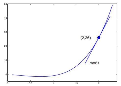
Figure \(\PageIndex{9}\): Graphs of \(F(t)=2 t^{4}-3 t\) and the line \(y = 61t − 96\).

Problem. Find an equation of the line tangent to the graph of

\[F(t)=\frac{1}{t^{2}} \quad \text { at the point } \quad(2,1 / 4)\]

Figure \(\PageIndex{10}\): A. Graphs of \(F(t)=1 / t^{2}\) and a secant to the graph through \(\left(b, 1 / b^{2}\right)\) and (2, 1/4). B. Graphs of \(F(t)=1 / t^{2}\) and the line \(y=-1 / 4 t+3 / 4\).

Solution. Graphs of \(F(t) = 1/t^2\) and a secant to the graph through the points \((b, 1/b^{2})\) and (2, 1/4) for a number \(b\) not equal to 2 are shown in Figure 3.1.10A.

The slope of the secant is

\[\begin{aligned}
\frac{F(b)-F(2)}{b-2} &=\frac{\frac{1}{b^{2}}-\frac{1}{2^{2}}}{b-2} \\
&=\frac{2^{2}-b^{2}}{b^{2} \cdot 2^{2}} \frac{1}{b-2} \\
&=-\frac{2+b}{2^{2} \cdot b^{2}} \quad \text { See Equation 3.1.19 }
\end{aligned}\]

We claim that

\[\text { As } b \text { approaches } 2, \quad \frac{F(b)-F(2)}{b-2}=-\frac{2+b}{2^{2} \cdot b^{2}} \quad \text { approaches } \quad-\frac{1}{4}\]

An equation of the line containing (2, 1/4) with slope -1/4 is

\[\frac{y-1 / 4}{t-2}=-1 / 4, \quad y=-\frac{1}{4} t+\frac{3}{4}\]

This is an equation of the line tangent to the graph of \[F(t)=1 / t^{2}\] at the point (2, 1/4). Graphs of \(F\) and \(y=-1 / 4 t+3 / 4\) are shown in Figure 3.1.10B.

Explore 3.1.7 In Explore Figure 3.1.7 is the graph of \(y=\sqrt[3]{x}\). Does the graph have a tangent at (0,0)? Your vote counts.

Explore Figure 3.1.7 Graph of \(y=\sqrt[3]{x}\)

Problem. At what rate is the function \(F(x)=\sqrt[3]{x}\) increasing at t = 8?

Solution. For a number b not equal to 8,

\[\begin{aligned}
&\frac{F(b)-F(8)}{b-8}=\frac{\sqrt[3]{b}-\sqrt[3]{8}}{b-8}\\
&=\frac{\sqrt[3]{b}-2}{(\sqrt[3]{b})^{3}-2^{3}} \quad \text { Lightning Bolt! See Figure 3.1.11 }\\
&=\frac{1}{(\sqrt[3]{b})^{2}+\sqrt[3]{b} \cdot 2+2^{2}}
\end{aligned}\]

Now we claim that

\[\text { as } b \text { approaches } 8 \quad \frac{F(b)-F(8)}{b-8}=\frac{1}{(\sqrt[3]{b})^{2}+\sqrt[3]{b} \cdot 2+2^{2}} \quad \text { approaches } \quad \frac{1}{12}\]

Therefore, the rate of increase of \(F(t)=\sqrt[3]{t}\) at t = 8 is 1/12. A graph of \(F(t)=\sqrt[3]{t}\) and \(y = t/12 + 4/3\) is shown in Figure 3.1.12.

Pattern. In each of the computations that we have shown, we began with an expression for

\[\frac{F(b)-F(a)}{b-a}\]

that was meaningless for \(b = a\) because of \(b − a\) in the denominator. We made some algebraic rearrangement that neutralized the factor \(b − a\) in the denominator and obtained an expression \(E(b)\) such that

1. \(\frac{F(b)-F(a)}{b-a}=E(b)\) for \(b \neq a\), and
2. \(E(a)\) is defined, and
3. As \(b\) approaches \(a\), \(E(b)\) approaches \(E(a)\)

A Lightning Bolt signals a step that is a surprise, mysterious, obscure, or of doubtful validity, or to be proved in later chapters. Think of Zeus atop Mount Olympus issuing thunderous proclamations amid darkness and lightning.

Figure \(\PageIndex{11}\): Figure of Zeus from http://en.wikipedia.org/wiki/Zeus. Picture is by Sdwelch1031

Figure \(\PageIndex{12}\): Graphs of \(F(t)=\sqrt[3]{t}\) and the line \(y = t/12 + 4/3\).

We then claimed that

\[\text { as } b \text { approaches } a \quad \frac{F(b)-F(a)}{b-a} \quad \text { approaches } \quad E(a) \text { . }\]

This pattern will serve you well until we consider exponential, logarithmic and trigonometric functions where more than algebraic rearrangement is required to neutralize the factor \(b − a\) in the denominator. Item 3 of this list is often given scant attention, but deserves your consideration.

Exercises for Section 3.1, Tangent to the graph of a function.

Exercise 3.1.1 Approximate the growth rate of the V. natriegens population of Table 1.1 at time t = 56 minutes.

Exercise 3.1.2 Approximate the growth rate of \(B(T) = 0.022\) at time a. T = 56 minutes, b. T = 30 minutes, c. T = 0 minutes.

Exercise 3.1.3 Shown in Exercise Figure 3.1.3 is the ventricular volume of the heart during a normal heart beat of 0.8 seconds. During systole the ventricle contracts and pushes the blood into the aorta. Find approximately the flow rate in ml/sec of blood in the aorta at time t = 0.2 seconds. Find approximately the maximum flow rate of blood in the aorta.

Figure for Exercise 3.1.3 Graph of the ventricular volume during a normal heart beat. Patterned after the graph in Figure 9.13.

Exercise 3.1.4 Shown in Exercise Figure 3.1.4 is a graph of air densities in \(kg/m^3\) as a function of altitude in meters (U.S. Standard Atmospheres 1976, National Oceanic and Atmospheric Administration, NASA, U.S. Air Force, Washington, D.C. October 1976). You will find the rate of change of density with altitude. Because the independent variable is altitude, a distance, the rate of change is commonly called the gradient.

1. At what rate is air density changing with increase of altitude at altitude = 2000 meters? Alternatively, what is the gradient of air density at 2000 meters?
2. What is the gradient of air density at altitude = 5000 meters?
3. What is the gradient of air density at altitude = 8000 meters?

Figure for Exercise 3.1.4 Graph of air density \((kg/m^{3})\) vs altitude (m)

Exercise 3.1.5 An African honey bee Apis mellifera scutellata was introduced into Brazil in 1956 by geneticists who hoped to increase honey production with a cross between the African bee which was native to the tropics and the European species commonly used by bee keepers in South America and in the United States. Twenty six African queens escaped into the wild in 1957 and the subsequent feral population has been very aggressive and has disrupted or eliminated commercial honey production in areas where they have spread.

Shown in Exercise Figure 3.1.5 is a map¹ that shows the regions occupied by the African bee in the years 1957 to 1983, and projections of regions that would be occupied by the bees during 1985-1995.

1. At what rate did the bees advance during 1957 to 1966?
2. At what rate did the bees advance during 1971 to 1975?
3. At what rate did the bees advance during 1980 to 1982?
4. At what rate was it assumed the bees would advance during 1983 - 1987?

Figure for Exercise 3.1.5 The spread of the African bee from Brazil towards North America. The solid curves with dates represent observed spread. The dashed curves and dates are projections of spread.

Exercise 3.1.6 If b approaches 3

1. \(b\) approaches __________.
2. \(2 \div b\) approaches __________. Note: Neither 0.6666 nor 0.6667 is the answer.
3. \(\pi\) approaches __________.
4. \(\frac{2}{\sqrt{b}+\sqrt{3}}\) approaches __________. Note: Neither 0.577 nor 0.57735026919 is the answer.
5. \(b^{3}+b^{2}+b\) approaches __________.
6. \(\frac{b}{1+b}\) approaches __________.
7. \(2^{b}\) approaches __________.
8. \(\log _{3} b\) approaches __________.

Exercise 3.1.7 In a classic study², David Ho and colleagues treated HIV-1 infected patients with ABT-538, an inhibitor of HIV-1 protease. HIV-1 protease is an enzyme required for viral replication so that the inhibitor disrupted HIV viral reproduction. Viral RNA is a measure of the amount of virus in the serum. Data showing the amount of viral RNA present in serum during two weeks following drug administration are shown in Table Ex. 3.1.7 for one of the patients. Before treatment the patients serum viral RNA was roughly constant at 180,000 copies/ml. On day 1 of the treatment, viral production was effectively eliminated and no new virus was produced for about 21 days after which a viral mutant that was resistant to ABT-538 arose. The rate at which viral RNA decreased on day 1 of the treatment is a measure of how rapidly the patient’s immune system eliminated the virus before treatment.

1. Compute an estimate of the rate at which viral RNA decreased on day 1 of the treatment.
2. Assume that the patient’s immune system cleared virus at that same rate before treatment. What percent of the virus present in the patient was destroyed by the patient’s immune system each day before treatment?
3. At what rate did the virus reproduce in the absence of ABT-538.

Table for Exercise 3.1.7 RNA copies/ml in a patient during treatment with an inhibitor of HIV-1 protease.

Observed
Time Days	RNA copies/ml Thousands
1	80
4	50
8	18
11	9.5
15	5

Exercise 3.1.8 Shown in Figure Ex. 3.1.8 is the graph of the line, \(y = 0.5 x\), and the point (2,1).

1. Is there a tangent to the graph of \(y = 0.5 x\) at the point (2,1)?
2. Suppose \(H(t) = 0.5 t\) is the height in feet of water above flood stage in a river \(t\) hours after midnight. At what rate is the water rising at time t = 2 am?

Figure for Exercise 3.1.8 Graph of the line \(y = 0.5x\). See Exercise 3.1.8.

Exercise 3.1.9 See Figure Ex. 3.1.9. Let A be the point (3,4) of the circle

\[x^{2}+y^{2}=25\]

Let B be a point of the circle different from A. What number does the slope of the line containing A and B approach as B approaches A?

Figure for Exercise 3.1.9 Graph of the circle \(x^{2}+y^{2}=25\) and a secant through (3,4) and a point B. See Exercise 3.1.9.

Exercise 3.1.10 Technology. Suppose plasma penicillin concentration in a patient following injection of 1 gram of penicillin is observed to be

\[P(t)=200 \cdot 2^{-0.03 t}\]

where \(t\) is time in minutes and \(P(t)\) is \(\mu g/ml\) of penicillin. Use the following steps to approximate the rate at which the penicillin level is changing at time t = 5 minutes and at t = 0 minutes.

1. t = 5 minutes. Draw the graph of \(P(t)\) vs \(t\) for \(4.9 \leq t \leq 5.1\). (The graph should appear to be a straight line on this short interval.)
2. Complete the table on the left, computing the average rates of change of penicillin level.

\(b\) \(\frac{P(b)-P(5)}{b-5}\) 4.9 -3.7521 4.95   4.99   4.995       5.005   5.01   5.05   5.1 -3.744

\(b\) \(\frac{P(b)-P(0)}{b-0}\) -0.1 OMIT -0.05 OMIT -0.01 OMIT -0.005 OMIT     0.005   0.01   0.05   0.1 -4.155

3. What is your best estimate of the rate of change of penicillin level at the time \(t = 5\) minutes? Include units in your answer.
4. t = 0 minutes. Complete the second table above. The OMIT entries in the second table refer to the fact that the level of penicillin, \(P(t)\), may not be given by the formula for negative values of time, \(t\). What is your best estimate of the rate of change of penicillin level at the time \(t = 0\) minutes?

Exercise 3.1.11 The patient in Exercise 3.1.10 had penicillin level 200 \(\mu g/ml\) at time t = 0 following a 1 gram injection. What is the approximate volume of the patient’s vascular pool? If you wished to maintain the patient’s penicillin level at 200 \(\mu g/ml\), at what rate would you continuously infuse the patient with penicillin?

Exercise 3.1.12 Find equations of the lines tangent to the graphs of the function F at the indicated points.

1. \(F(t)=t^{2}\) at (2, 4)
2. \(F(t)=t^{2}+2\) at (2, 6)
3. \(F(t)=t+1\) at (2, 3)
4. \(F(t)=3 t^{3}-4 t^{2}\) at (1, -1)
5. \(F(t)=1 /(t+1)\) at (1, 1/2)
6. \(F(t)=\sqrt[4]{t}\) at (1, 1)

Exercise 3.1.13 Find the rates of change of the function F at the indicated points.

a. \(F(t)=t^{3}\) at (2, 8)
b. \(F(t)=1 / t\) at (2, 1/2)
c. \(F(t)=2 t+t^{2}\) at (2,8)
d. \(F(t)=\sqrt{t}\) at (4, 2)
e. \(F(t)=t /(t+1)\) at (1, 1/2)
f. \(F(t)=(t+1) / t\) at (1, 2)

Figure for Exercise 3.1.14 A parabola with vertex at A and a secant through A and a point B. See Exercise 3.1.14.

 

¹ Orley R. Taylor, African bees: potential impact in the United States, Bull Ent Soc of America, Winter, 1985, 15-24. Copyright, 1985, The Entomological Society of America.

² David D. Ho, Avidan U Neumann, Alan S. Perlson, Wen Chen, John M. Leonard, & Martin Markowitz, Rapid turnover of plasma virions and CD4 lymphocytes in HIV-1 infection, Nature 373, 123-126, (1995)