4.1: Continuity

Most, but not all, of the functions in previous sections and that you will encounter in biology are continuous. Four equivalent definitions of continuity follow, with differing levels of intuition and formality.

Definition 4.1.1 Continuity of a function at a number in its domain.

Intuitive: A function, \(f\), is continuous at a number \(a\) in its domain means that if \(x\) is in the domain of \(f\) and \(x\) is close to \(a\), then \(f(x)\) is close to \(f(a)\).

Symbolic: A function, \(f\), is continuous at a number a in its domain means that either

\[\lim _{x \rightarrow a} f(x) = f(a)\]

or there is an open interval containing a and no other point of the domain of f.

Formal: A function, \(f\), is continuous at a number \(a\) in its domain means that for every positive number, \(\epsilon\), there is a positive number \(\delta\) such that if \(x\) is in the domain of \(f\) and \(|x − a| < \delta\) then \(|f(x) − f(a)| < \epsilon\).

Geometric A simple graph \(G\) is continuous at a point \(P\) of \(G\) means that if \(\alpha\) and \(\beta\) are horizontal lines with \(P\) between them there are vertical lines \(h\) and \(k\) with \(P\) between them such that every point of of \(G\) between \(h\) and \(k\) is between \(\alpha\) and \(\beta\).

Definition 4.1.2 Discontinuous. If \(a\) is a number in the domain of a function \(f\) at which \(f\) is not continuous then \(f\) is said to be discontinuous at \(a\).

Definition 4.1.3 Continuous function. A function, \(f\), is continuous means that \(f\) is continuous at every number, \(a\), in its domain.

Explore 4.1.1. Definition 4.1.2 is a sleeper. What does "not continuous" mean? It is a rite of passage for mathematics students to write the negation of the statement that a function is continuous at a number \(a\) in its domain. The statement is sometimes called the "logical complement" or the "bare denial" of the statement of continuity at \(a\). To illustrate, the negation of the Symbolic Definition is

Symbolic Definition of Discontinuity: A function, \(f\), which has a number \(a\) in its domain is not continuous at a means that every open interval containing a contains a point of the domain of \(f\) different from \(a\) and either

\[\lim _{x \rightarrow a} f(x) \text { does not exist, } \quad \text { or } \quad \lim _{x \rightarrow a} f(x) \quad \text { exists and is not }=f(a) \text {. }\]

The Intuitive Definition is so imprecise as to make its negation even more difficult. You should try to write that negation, but will likely first write, "There is a number, \(x\), close to \(a\) for which \(f(x)\) is not close to \(f(a)\)," but this suffers from the uncertainty of "close to."

Explore 4.1.2 Write the negation of the Formal Definition of Continuity of a function, \(f\), at a point, \(a\), of its domain. This is something into which you can sink your teeth, deeply.

As a guide, we write a negation of the Geometric Definition of continuity.

Geometric Definition of Discontinuity: A simple graph \(G\) that contains a point \(P\) is not continuous \(P\) means that there are horizontal lines \(\alpha\) and \(\beta\) with \(P\) between them such that for any are vertical lines \(h\) and \(k\) with \(P\) between them some point of of \(G\) between \(h\) and \(k\) is not between \(\alpha\) and \(\beta\).

Most of the functions that you have experienced are continuous, and to many students it is intuitively obvious from the notation that \(u(b)\) approaches \(u(a)\) as \(b\) approaches \(a\); but in some cases \(u(b)\) does not approach \(u(a)\) as \(b\) approaches \(a\). Some examples demonstrating both continuity and discontinuity follow.

Example 4.1.1

1. You showed in Exercise 3.2.7 that every polynomial is continuous.
2. The function describing serum insulin concentration as a function of time is a continuous function even though it may change quickly with serious consequences.
3. The word 'threshold' suggests a discontinuous change in one parameter as a related parameter crosses the threshold. Stimulus to neurons causes ion gates to open. When an Na+ ion gate is opened, Na\(^{+}\) flows into the cell gradually increasing the membrane potential, called a 'graded response' (continuous response), up to a certain threshold at which an action potential is triggered (a rapid increase in membrane potential) that appears to be a discontinuous response. As in almost all biological examples, however, the function is actually continuous. See Example Figure 4.1.1.1A.
4. Surprise. The graph in Figure 4.1.1.1B is continuous. There are only three points of the graph. The graph is continuous at, for example, the point (3,2). There is an open interval containing 3, (2.7, 3.3), for example, that contains 3 and no other point of the domain.

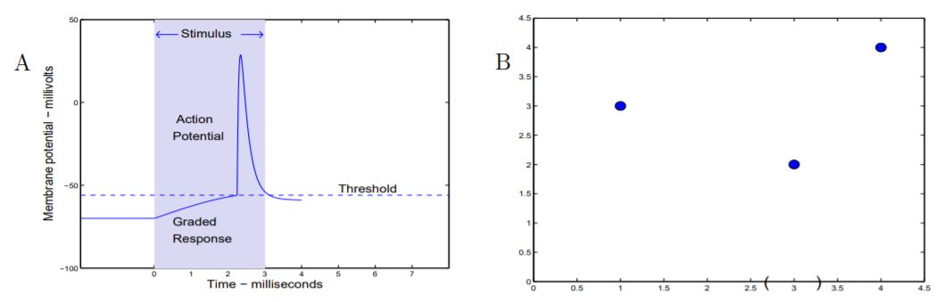
Figure for Example 4.1.1.1 A. Events leading to a nerve action potential. B. A discrete graph is continuous.

5. The function approximating % Female hatched from a clutch of turtle eggs \[\text { Percent female }=\left\{\begin{array}{lll}
   0 & \text { if }  &\text { Temp} & < \quad 28 \\
   50 & \text { if }  &\text { Temp} & = \quad 28 \\
   100 & \text { if }  & \quad 28 & < \quad \text{Temp }
   \end{array}\right. \label{4.1}\] is not continuous. The function is discontinuous at \(t = 28\). If the temperature, \(T\), is close to 28 and less than 28, then % Female(T) is 0, which in usual measures is not 'close to' 50 = % Female(28).
6. As you move up a mountain side, the flora is usually described as being a discontinuous function of altitude. There is a 'tree line', below which the dominant plant species are pine and spruce and above which the dominant plant species are low growing brushes and grasses, as illustrated in Figure 4.1.1.1C¹

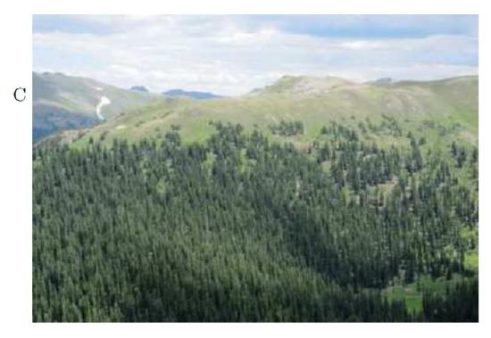
Figure for Example 4.1.1.1 (Continued.) C. A tree line. Picture taken from the summit of Independence Pass, Colorado at 12,095 feet (3687 m) elevation.

7. We acknowledge that the tree line in Figure 4.1.1.1 is not sharp and some may not agree that it marks a discontinuity.

It is important to the concept of discontinuity that there be an abrupt change in the dependent variable with only a gradual change in the independent variable. Charles Darwin expressed it:

Charles Darwin, Origin of Species. Chap. VI, Difficulties of the Theory. “We see the same fact in ascending mountains, and sometimes it is quite remarkable how abruptly, as Alph. de Candolle has observed, a common alpine species disappears. The same fact has been noticed by E. Forbes in sounding the depths of the sea with the dredge. To those who look at climate and the physical conditions of life as the all-important elements of distribution, these facts ought to cause surprise, as climate and height or depth graduate away insensibly [our emphasis].”

8. From Equation 3.2.28, \(\lim _{x \rightarrow a} \frac{1}{x} = \frac{1}{a}\), the function, \(f(x) = \frac{1}{x}\) is continuous. The graph of \(f(x)\) certainly changes rapidly near \(x = 0\), and one may think that \(f\) is not continuous at \(x = 0\). However, 0 is not in the domain of \(f\), so that the function is neither continuous nor discontinuous at \(x = 0\).
9. Let the function \(g\) be defined by \[g(x)=\frac{1}{x} \quad \text { for } \quad x \neq 0, \quad g(0)=2\] A graph of \(g\) is shown in Example Figure 4.1.1.1E. The function \(g\) is not continuous at 0 and the graph of \(g\) is not continuous at (0, 2). Two horizontal lines above and below (0, 2) are drawn in Figure 4.1.1.1F. For every pair of vertical lines \(h\) and \(k\) with (0, 2) between them there are points of the graph of \(g\) between \(h\) and \(k\) that are not between \(\alpha\) and \(\beta\).

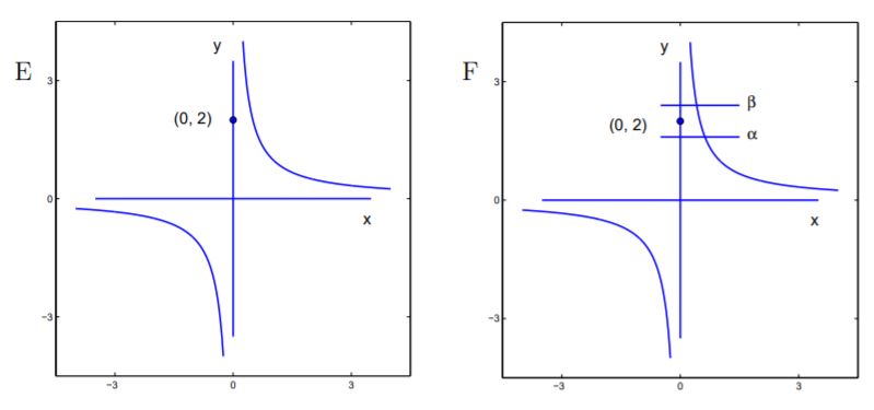
Figure for Example 4.1.1.1 (Continued) E. The graph of \(g(x) = 1/x\) for \(x \neq 0\), \(g(0) = 2\). F. The point (0, 2) and horizontal lines above and below (0, 2).

Explore 4.1.3 In Figure 4.1.1 there are two vertical dashed lines with (0,2) between them. It appears that every point of the graph of \(g\) between the vertical dashed lines is between the two horizontal lines. Does this contradict the claim made in Item 9?

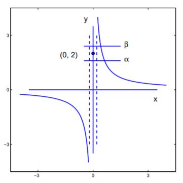
Explore Figure 4.1.1 The graph of \(g(x) = 1/x\) for \(x \neq 0\), \(g(0) = 2\), horizontal lines above and below (0, 2), and vertical lines (dashed) with (0, 2) between them.

10. The geological age of soil is not a continuous function of depth below the surface. Older soils are at a greater depth, so that the age of soils is (almost always) an increasing function of depth. However, in many locations, soils of some ages are missing: soils of age 400 million years may rest directly on top of soils of age 1.7 billion years as shown in Figure 4.1.1.1. Either soils of the intervening ages were not deposited in that location or they were deposited and subsequently eroded. Geologist speak of an "unconformity" occurring at that location and depth.

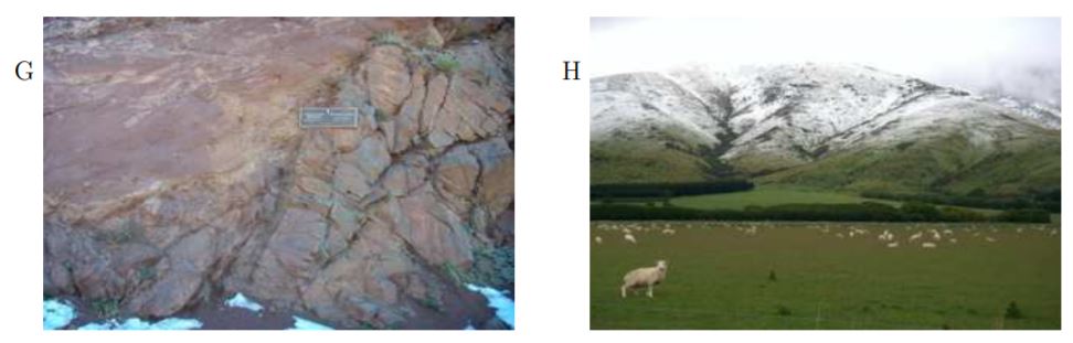
Figure for Example 4.1.1.1 (Continued) G. Picture of an unconformity at Red Rocks Park and Amphitheatre near Denver, Colorado. Red 300 million year-old sedimentary rocks rest on gray 1.7 billion year-old metamorphic rocks. (Better picture in ”Messages in Stone: Colorado’s Colorful Geology” Vincent Matthews, Katie KellerLynn, and Betty Fox, Colorado Geological Survey, Denver, Colorado, 2003) H. Snow line figure taken in New Zealand for Exercise 4.1.4.

11. Every increasing function defined on an interval that is discontinuous at some point has a vertical gap in the graph at that point. Every increasing function with no gap is continuous. Vertical gap: there is a horizontal line that does not intersect the graph, but has a point of the graph below the line and a point of the graph above the line.

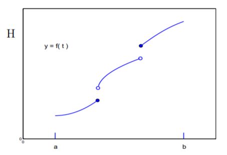
Figure for Example 4.1.1.1 (Continued) H. An increasing function. There are two vertical gaps and two points of discontinuity.

Explore 4.1.4 Vertical gap in the graph G means an interval of the Y-axis that contains no point of the Y-projection of G and for which there is a point of the Y-projection of G below the interval and a point of the Y-projection of G above the interval. Is there a continuous and increasing function that has a vertical gap?

Combinations of continuous functions. We showed in Chapter 3 that

\[\begin{aligned}
\lim _{x \rightarrow a}\left(F_{1}(x)+F_{2}(x)\right)=\lim _{x \rightarrow a} F_{1}(x)+\lim _{x \rightarrow a} F_{2}(x) \quad & \text{Equation 3.14} \\
\lim _{x \rightarrow a}\left(F_{1}(x) \times F_{2}(x)\right)=\left(\lim _{x \rightarrow a} F_{1}(x)\right) \times\left(\lim _{x \rightarrow a} F_{2}(x)\right) \quad & \text{Equation 3.15} \\
\text{If} \quad \lim _{x \rightarrow a} F_{2}(x) \neq 0, \quad \text{then} \quad \lim _{x \rightarrow a} \frac{F_{1}(x)}{F_{2}(x)}=\frac{\lim _{x \rightarrow a} F_{1}(x)}{\lim _{x \rightarrow a} F_{2}(x)} \quad & \text{Equation 3.18} \\
\end{aligned}\]

From these results it follows that if \(u\) and \(v\) are continuous functions with common domain, \(D\), then

\[u+v \quad \text { and } \quad u \times v \quad \text { are continuous, } \label{4.2}\]

and if \(v(t)\) is not zero for any \(t\) in \(D\), then

\[\frac{u}{v} \quad \text{is continuous} \label{4.3}\]

Of particular interest is the equation on the limit of composition of two functions,

\[\text { If } \lim _{x \rightarrow a} u(x)=L \quad \text { and } \quad \lim _{s \rightarrow L} F(s)=\lambda, \quad \text { then } \quad \lim _{x \rightarrow a} F(u(x))=\lambda, \quad \text { Equation } 3.17\]

From this it follows that if \(F\) and \(u\) are continuous and the domain of \(F\) contains the range of \(u\) then

\[F \circ u, \quad \text { the composition of } F \text { with } u \text {, is continuous. } \label{4.4}\]

 

Exercises for Section 4.1, Continuity.

Exercise 4.1.1

1. Find an example of a plant ecotone distinct from the tree line example shown in Figure 4.1.1.1.
2. Find an example of a discontinuity of animal type.

Exercise 4.1.2 For \(f(x) = 1/x\),

1. How close must \(x\) be to 0.5 in order that \(f(x)\) is within 0.01 of 2?
2. How close must \(x\) be to 3 in order to insure that \(\frac{1}{x}\) be within 0.01 of \(\frac{1}{3}\) ?
3. How close must \(x\) be to 0.01 in order to insure that \(\frac{1}{x}\) be within 0.1 of 100?

Exercise 4.1.3 Find the value for \(u(2)\) that will make \(u\) continuous if

1. \(u(t) = 2t + 5\) for \(t \neq 2\)
2. \(u(t) = \frac{t ^{2} − 4}{t − 2}\) for \(t \neq 2\)
3. \(u(t) = \frac{(t − 2)^2}{|t − 2|}\) for \(t \neq 2\)
4. \(u(t) = \frac{t + 1}{t − 3}\) for \(t \neq 2\)
5. \(u(t) = \frac{t − 2}{t ^{3} − 8}\) for \(t \neq 2\)
6. \(u(t) = \frac{\frac{1}{t} − \frac{1}{2}}{t − 2}\) for \(t \neq 2\)

Exercise 4.1.4 In Example Figure 4.1.1.1 H is a picture of snow that fell on the side of a mountain the night before the picture was taken. There is a 'snow line', a horizontal separation of the snow from terrain free of snow below the line. 'Snow' is a discontinuous function of altitude. Explain the source of the discontinuity.

Exercise 4.1.5 a. Draw the graph of \(y_1\). b. Find a number \(A\) such that the graph of \(y_2\) is continuous.

1. \(\quad y_{1}(x)=\left\{\begin{array}{r}x^{2} \quad \text { for } \quad x<2 \\ 3-x \quad \text { for } \quad 2 \leq x\end{array}\right.\)
2. \(\quad y_{2}(x)=\left\{\begin{array}{r}x^{2} \quad \text { for } \quad x<2 \\ A-x \quad \text { for } \quad 2 \leq x\end{array}\right.\)

Exercise 4.1.6 Is the temperature of the water in a lake a continuous function of depth? Write a paragraph discussing water temperature as a function of depth in a lake and how knowledge of water temperature assists in the location of fish.

Exercise 4.1.7 To reduce inflammation in a shoulder, a doctor prescribes that twice daily one Voltaren tablet (25 mg) to be taken with food. Draw a graph representative of the amount of Voltaren in the body as a function of time for a one week period. Is your graph continuous?

Exercise 4.1.8 The function, \(f(x) = \sqrt[3] x\) is continuous.

1. How close must \(x\) be to 1 in order to insure that \(f(x)\) is within 0.1 of \(f(1) = 1\) (that is, to insure that \(0.9 < f(x) < 1.1\))?
2. How close must \(x\) be to 1/8 in order to insure that \(f(x)\) is within 0.0001 of \(f(1/8) = 1/2\) (that is, to insure that \(0.4999 < f(x) < 0.5001\))?
3. How close must \(x\) be to 0 in order to insure that \(f(x)\) is within 0.1 of \(f(0) = 0\)?

Exercise 4.1.9

1. Draw the graph of a function, \(f\), defined on the interval [1, 3] such that \(f(1) = −2\) and \(f(3) = 4\).
2. Does your graph intersect the X-axis?
3. Draw a graph of of a function, \(f\), defined on the interval [1, 3] such that \(f(1) = −2\) and \(f(3) = 4\) that does not intersect the X-axis. Be sure that its X-projection is all of [1, 3].
4. Write equations to define a function, \(f\), on the interval [1, 3] such that \(f(1) = −2\) and \(f(3) = 4\) and the graph of \(f\) does not intersect the X-axis.
5. There is a theorem that asserts that the function you just defined must be discontinuous at some number in [1,3]. Identify such a number for your example.

The preceding exercise illustrates a general property of continuous functions called the intermediate value property. Briefly it says that a continuous function defined on an interval that has both positive and negative values on the interval, must also be zero somewhere on the interval. In language of graphs, the graph of a continuous function defined on an interval that has a point below the X-axis and a point above the X-axis must intersect the X-axis. The proof of this property requires more than the familiar properties of addition, multiplication, and order of the real numbers. It requires the completion property of the real numbers, Axiom 5.2.1².

Exercise 4.1.10 A nutritionist studying plasma epinephrine (EPI) kinetics with tritium labeled epinephrine, [³H]EPI, observes that after a bolus injection of [³H]EPI into plasma, the time-dependence of [³H]EPI level is well approximated by \(L(t) = 4e ^{−2t} + 3e ^{−t}\) where \(L(t)\) is the level of [³H]EPI \(t\) hours after infusion. Sketch the graph of \(L\). Observe that \(L(0) = 7\) and \(L(2) = 0.479268\). The intermediate value property asserts that at some time between 0 and 2 hours the level of [³H]EPI will be 1.0. At what time, \(t_1\), will \(L(t_{1}) = 1.0\)? (Let \(A = e ^{−t}\) and observe that \(A^{2} = e ^{−2t}\).)

Exercise 4.1.11 For the function, \(f(x) = 10 − x ^{2}\), find an an open interval, \((3 − \delta, 3 + \delta)\) so that \(f(x) > 0\) for \(x\) in \((3 − \delta, 3 + \delta)\).

Exercise 4.1.12 For the function, \(f(x) = \sin (x)\), find an an open interval, \((3 − \delta, 3 + \delta)\) so that \(f(x) > 0\) for \(x\) in \((3 − \delta, 3 + \delta)\).

Exercise 4.1.13 The previous two problems illustrate a property of continuous functions formulated in the Locally Positive Theorem:

Theorem 4.1.1 Locally Positive Theorem. If a function, \(f\), is continuous at a number \(a\) in its domain and \(f(a)\) is positive, then there is a positive number, \(\delta\), such that \(f(x)\) is positive for every number \(x\) in \((a − \delta, a + \delta)\) and in the domain of \(f\).

Prove the Locally Positive Theorem. Your proof may begin:

1. Suppose the hypothesis of the Locally Positive Theorem.
2. Let \(\epsilon = f(a)\).
3. Use the hypothesis that \(\lim _{x \rightarrow a} f(x) = f(a)\).

Exercise 4.1.14 Is it true that if a function, \(f\), is positive at a number \(a\) in its domain, then there is a positive number, \(\delta\), such that if \(x\) is in \((a − \delta, a + \delta)\) and in the domain of \(f\) then \(f(x) > 0\)?

 

¹ Such a region of apparent discontinuity is termed an 'ecotone' by ecologists.

² The intermediate value property is equivalent to the completion property within the usual axioms of the number system. See Exercise 12.1.8