
4.5: Some optimization problems.


- Last updated
- Jan 1, 2022
- Save as PDF
( \newcommand{\kernel}{\mathrm{null}\,}\)
In Section 3.5.2 we found that local maxima and minima are often points at which the derivative is zero. The algebraic functions for which we can now compute derivatives have only a finite number of points at which the derivative is zero or does not exist and it is usually a simple matter to search among them for the highest or lowest points of their graphs. Such a process has long been used to find optimum parameter values and a few of the traditional problems that can be solved using the derivative rules of this chapter are included here. More optimization problems appear in Chapter 8 Applications of the Derivative.
Assume for this section only that all local maxima and local minima of a function,
Example 4.5.1 A forester needs to get from point
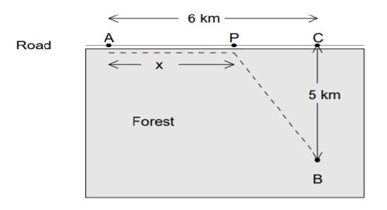
Figure
Solution. She might go directly from
Assume that the road is straight, the distance from
so that
The distance traveled and time required are
The total trip time,
A graph of
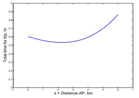
Figure
Explore 4.5.1 It appears that to minimize the time of the trip, the forester should travel about 2.5 km along the road from
Compute the derivative of
Note: The constant denominators may be factored out, as in
You should get
Find the value of
Your conclusion should be that the forester should travel 2.25 km from
Exercises for Section 4.5, Some optimization problems.
Exercise 4.5.1 In Example 4.5.1, what should be the path of the forester if she can travel 10 km/hr on the road and 4 km/hr in the forest?
Exercise 4.5.2 The air temperature is
where:
Assume that if she travels at a speed,
- At what speed should she travel in order to minimize the amount of body heat that she looses during the 10 mile bicycle ride?
- Frostbite is skin tissue damage caused by prolonged skin tissue temperature of
- Discuss her options if the ambient air temperature is
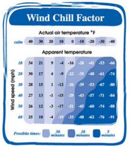
Figure for Exercise 4.5.2 Table of windchill temperatures for values of ambient air temperatures and wind speeds provided by the Center for Disease Control at http://emergency.cdc.gov/disasters/winter/pdf/cold guide.pdf. It was adapted from a more detailed chart at http://www.nws.noaa.gov/om/windchill.
Exercise 4.5.3 If
bushels per acre. Corn is worth $6.50 per bushel and nitrogen costs $0.63 per pound. All other costs of growing and harvesting the crop amount to $760 per acre, and are independent of the amount of nitrogen fertilizer applied. How much nitrogen per acre should be used to maximize the net dollar return per acre? Note: The parameters of this problem are difficult to keep up to date.
Exercise 4.5.4 Optimum cross section of your femur. R. M. Alexander3 has an interesting analysis of the cross section of mammal femurs. Femurs are hollow tubes filled with marrow. They should resist forces that tend to bend them, but not be so massive as to impair movement. An optimum femur will be the lightest bone that is strong enough to resist the maximum bending moment,
A hollow tube of mass
The constant
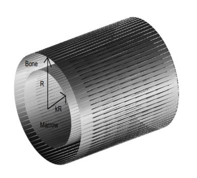
Figure
Let
- Write an equation for the mass per unit length of the bone marrow similar to Equation
- Let
- Find a value of
- The value
- Exercise Figure 4.5.4B is a cross section of the human leg at mid-thigh. Estimate x for the femur.
Alexander modifies this result, noting that Equation 4.13 is the breaking moment, and a bone with walls this thin would buckle before it broke, and noting that bones are tapered rather than of uniform width.
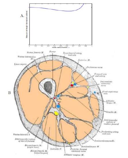
Figure for Exercise 4.5.4 A. Graph of Equation
3 R. McNeil Alexander, Optima for Animals, Princeton University Press, Princeton, NJ, 1996, Section 2.1, pp 17-22.