5.4: The derivative of \(e ^{k t}\).

We have found the derivative of \(e ^t\). Often, however, the function of interest is of the form \(C ~ e^{k t}\) where \(C\) and \(k\) are constants. In Example 5.3.1 of bacterial growth,

\[\text { Abs }=0.0174 e^{0.02176 \text { Time }}\]

the constant \(C = 0.0174\) and the function \(k t = 0.02176\) Time. We develop a formula for \(\left[e^{k t}\right]^{\prime}\).

\[\begin{array}\
{\left[e^{k t}\right]^{\prime} } &=\left[\left(e^{t}\right)^{k}\right]^{\prime} & (i)\\
&=k\left(e^{t}\right)^{k-1}\left[e^{t}\right]^{\prime} & (ii)\\
&=k\left(e^{t}\right)^{k-1} e^{t} & (iii)\\
&=k e^{k t} &\\
\end{array} \label{5.15}\]

Because Equation \ref{5.15} \(\left[e^{k t}\right]^{\prime}=k e^{k t}\), is used so often, we call it another Primary Formula even though we developed it without direct reference to the Definition of Derivative. Should you be limited to a single derivative rule, in the life sciences choose the \(e ^{k t}\) Rule – exponential functions are ubiquitous in biology.

\(e^{kt}\) Rule

\[E(t)=e^{k t} \quad \Rightarrow \quad E^{\prime}(t)=e^{k t} k \quad\left[\mathbf{e}^{\mathbf{k t}}\right]^{\prime}=\mathbf{k} \mathbf{e}^{\mathbf{k t}} \label{5.16}\]

Explore 5.4.1 Were we to derive \(\left[e^{k t}\right]^{\prime}=k e^{k t}\)

\[\begin{array}\
{\left[e^{k t}\right]^{\prime} } &=\lim _{b \rightarrow a} \frac{e^{k b}-e^{k a}}{b-a} & (i)\\
&=\lim _{b \rightarrow a} \frac{e^{k b}-e^{k a}}{k b-k a} k & (ii)\\
&=e^{k a} k & (iii)\\
\end{array} \label{5.17}\]

The assertion in step (iii) that

\[\lim _{b \rightarrow a} \frac{e^{k b}-e^{k a}}{k b-k a}=e^{k a}\]

is correct, puzzles some students, and is worth your thought.

We can now differentiate functions like \(P(t)=5 t^{7}+3 e^{2 t}\).

\[\begin{aligned}
P^{\prime}(t) &=\left[5 t^{7}+3 e^{2 t}\right]^{\prime} & \text{A symbolic identity.}\\
&=\left[5 t^{7}\right]^{\prime}+\left[3 e^{2 t}\right]^{\prime} & \text{Sum Rule}\\
&=5\left[t^{7}\right]^{\prime}+3\left[e^{2 t}\right]^{\prime} & \text{Constant Factor Rule}\\
&=5 \times 7 t^{6}+3\left[e^{2 t}\right]^{\prime} & \text{Power Rule}\\
&=35 t^{6}+3 e^{2 t} 2 & e^{k t} \text{ Rule}\\
&=35 t^{6}+6 e^{2 t}\\
\end{aligned}\]

Example 5.4.1 We can also compute \(E ^{\prime} (t)\) for \(E(t) = 2^t\).

\[\left[2^{t}\right]^{\prime}=\left[\left(e^{\ln 2}\right)^{t}\right]^{\prime}=\left[e^{(\ln 2) t}\right]^{\prime}=e^{(\ln 2) t} \ln 2=2^{t} \ln 2\]

We have an exact solution for the first problem of this Chapter, which was to find \(E ^{\prime} (2)\) for \(E(t) = 2^t\). The answer is \(2^2 \ln {2} = 4 \ln {2}\). Also, \(E ^{\prime} (0) = 2^{0} \ln {2} = \ln {2}\) which answers another question from early in the chapter.

More generally, for \(b > 0\),

\[\begin{array}\
{\left[b^{t}\right]^{\prime} } &=\left[\left(e^{\ln b}\right)^{t}\right]^{\prime} & (i) \\
&=\left[e^{(\ln b) t}\right]^{\prime} & (ii)\\
&=e^{(\ln b) t} \ln b & (iii)\\
&=b^{t} \ln b & (iv)\\
\end{array} \label{5.18}\]

We summarize this information:

\[\left[b^{t}\right]^{\prime}=b^{t} \ln b \quad \text { for } b>0\]

Explore 5.4.2 This is very important. Show that if \(C\) and \(k\) are constants and \(P(t) = C~e^{k t}\) then \(P ^{\prime} (t) = k~P(t)\).

 

Exercises for Section 5.4, The derivative of \(e ^{k t} \).

Exercise 5.4.1 Give reasons for the steps (i) − (iii) in Equation \ref{5.15} showing that \(\left[e^{k t}\right]^{\prime}=e^{k t} k\).

Exercise 5.4.2 Give reasons for the steps (i) − (iv) in Equation \ref{5.18} showing that \(\left[b^{t}\right]^{\prime}=b^{t} \ln b\).

Exercise 5.4.3 The function \(b ^t\) for \(b = 1\) is a special exponential function. Confirm that the derivative equation \(\left[b^{t}\right]^{\prime}=b^{t} \ln b\) is valid for \(b = 1\). Draw some graphs of \(b ^t\) for \(b = 1\) and its derivative.

Exercise 5.4.4 Use one rule for each step and identify the rule to differentiate

1. \(P(t)=3 e^{5 t}+\pi\)
2. \(P(t)=\frac{e^{2}}{2}+\frac{t^{3}}{3}\)
3. \(P(t)=5^{t}\)
4. \(P(t)=e^{2 t} e^{3 t}\)

Simplify Part d before differentiating.

Exercise 5.4.5 Compute \(y ^{\prime} (x)\) or assert that you do not yet have forumlas to compute \(y ^{\prime} (x)\) for

1. \(y(x)=e^{5 x}\)
2. \(y(x)=e^{-3 x}\)
3. \(y(x)=e^{\sqrt{x}}\)
4. \(y(x)=\left(e^{x}\right)^{2}\)
5. \(y(x)=\left(e^{\sqrt{x}}\right)^{2}\)
6. \(y(x)=\left(e^{-x}\right)^{2}\)
7. \(y(x)=\frac{e^{x}+e^{-x}}{2}\)
8. \(y(x)=\frac{e^{x}-e^{-x}}{2}\)
9. \(y(x)=5 e^{-0.06 x}+3 e^{-0.1 x}\)
10. \(y(x)=e^{\left(x^{2}\right)}\)
11. \(y(x)=\sqrt{e^{x}}\)
12. \(y(x)=8 e^{-0.0001 x}-16 e^{-0.001 x}\)
13. \(y(x)=e^{5}\)
14. \(y(x)=\sqrt{e}\)
15. \(y(x)=10^{x}\)
16. \(y(x)=10^{-x}\)
17. \(y(x)=x^{2}+2^{x}\)
18. \(y(x)=\left(e^{5 x}+e^{-3 x}\right)^{5}\)

Exercise 5.4.6 Interpret \(e ^{t ^{2}}\) as \(e ^{(t ^{2} )}\) . Argue that

\[\lim _{b \rightarrow a} \frac{e^{\left(b^{2}\right)}-e^{\left(a^{2}\right)}}{b^{2}-a^{2}}=e^{\left(a^{2}\right)}\]

What is the ambiguity in the notation \(e ^{a ^{2}}\). (Consider \(4^{3^{2}}\).) Use parenthesis, they are cheap. However, common practice is to interpret (e ^{t ^{2}}\) as \(e ^{(t ^{2} )}\).

Exercise 5.4.7 Argue that

\[\lim _{b \rightarrow a} \frac{e^{\sqrt{b}}-e^{\sqrt{a}}}{\sqrt{b}-\sqrt{a}}=e^{\sqrt{a}}\]

Exercise 5.4.8 Review the method in Explore 5.4.1 and the results in Exercises 5.4.6 and 5.4.7. Use Definition 3.22,

\[F^{\prime}(a)=\lim _{b \rightarrow a} \frac{F(b)-F(a)}{b-a}, \quad \text { to compute } E^{\prime}(a) \text { for }\]

1. \(E(t)=e^{2 t}\)
2. \(E(t)=e^{2 \sqrt{t}}\)
3. \(E(t)=e^{-t}\)
4. \(E(t)=e^{2}\)
5. \(E(t)=e^{\frac{1}{t}}\)
6. \(E(t)=e^{-t^{2}}\)

Exercise 5.4.9 Consider the kinetics of penicillin that is taken as a pill in the stomach. The diagram in Figure Ex. 5.4.9(a) may help visualize the kinetics. We will find in Chapter 17 that a model of plasma concentration of antibiotic \(t\) hours after ingestion of an antibiotic pill yields an equation similar to

\[C(t)=5 e^{-2 t}-5 e^{-3 t} \quad \mu \mathrm{g} / \mathrm{ml}\]

A graph of \(C\) is shown in Figure Ex. 5.4.9. At what time will the concentration reach a maximum level, and what is the maximum concentration achieved?

As we saw in Section 3.5.2 and may be apparent from the graph in Figure Ex. 5.4.9, the highest concentration is associated with the point of the graph of \(C\) at which \(C ^{\prime} = 0\); the tangent at the high point is horizontal. The question, then, is at what time \(t\) is \(C ^{\prime} (t) = 0\) and what is \(C(t)\) at that time?

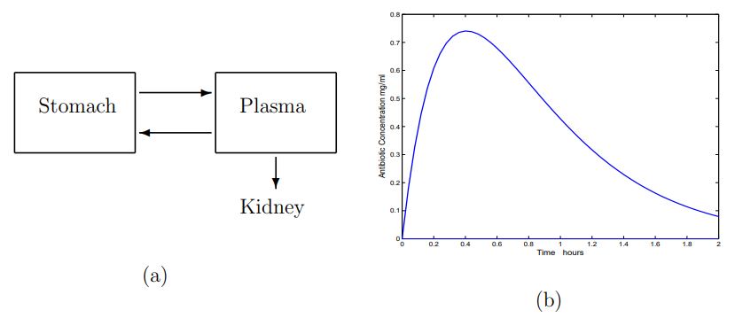
Figure for Exercise 5.4.9 (a) Diagram of compartments for oral ingestion of penicillin. (b) Graph of \(C(t)=5 e^{-2 t}-5 e^{-3 t}\) representative of plasma penicillin concentration \(t\) minutes after ingestion of the pill.

Exercise 5.4.10 Plasma penicillin concentration is

\[P(t)=5 e^{-0.3 t}-5 e^{-0.4 t}\]

\(t\) hours after ingestion of a penicillin pill into the stomach. A small amount of the drug diffuses into tissue and the tissue concentration, \(C(t)\), is

\[C(t)=-e^{-0.3 t}+0.5 e^{-0.4 t}+0.5 e^{-0.2 t} \quad \mu \mathrm{g} / \mathrm{ml}\]

1. Use your technology (calculator or computer) to find the time at which the concentration of the drug in tissue is maximum and the value of \(C\) at that time.
2. Compute \(C ^{\prime} (t)\) and solve for \(t\) in \(C ^{\prime} (t) = 0\). This is really bad, for you must solve for t in \[0.3 e^{-0.3 t}-0.2 e^{-0.4 t}-0.1 e^{-0.2 t}=0\] Try this: \[\text { Let } \quad Z=e^{-0.1 t} \quad \text { then solve } \quad 0.3 Z^{3}-0.2 Z^{4}-0.1 Z^{2}=0\].
3. Solve for the possible values of \(Z\). Remember that \(Z = e ^{-0.1 t}\) and solve for \(t\) if possible using the possible values of \(Z\).
4. Which value of \(t\) solves our problem?