
6.1: Derivatives of Products and Quotients.
- Page ID
- 36866

Derivatives of products. We determine the derivative of a function, \(P\), that is a product of two functions, \(P(t) = u(t) \times v(t)\) in terms of the values of \(u(t), u ^{\prime} (t), v(t)\) and \(v ^{\prime} (t)\); all four are required. The formula we obtain is
\[[u(t) \times v(t)]^{\prime}=u^{\prime}(t) \times v(t)+u(t) \times v^{\prime}(t) \label{6.2}\]
It is not a very intuitive formula. The derivative of a sum of two functions is the sum of the derivatives of the functions. One might expect derivative of the product of two functions to be the product of the derivatives of the two functions. Alas, this is seldom correct, but were it correct your learning of calculus would be notably simplified.
The correct formula is used as follows. Let
\[P(t)=t^{3} \times e^{-2 t}\]
Then with \(u(t) = t ^3\) and \(v(t) = e ^{-2t}\),
\[\begin{aligned}
P^{\prime}(t) &=\left[t^{3}\right]^{\prime} \times e^{-2 t}+t^{3} \times\left[e^{-2 t}\right]^{\prime} \\
&=3 t^{2} \times e^{-2 t}+t^{3} \times e^{-2 t} \times(-2)
\end{aligned}\]
A product of functions is useful, for example, in examining the factors affecting total corn production. Total production, \(P(t)\), is the product of the number of acres planted, \(A(t)\), and the average yield per acre, \(Y (t)\). The factors that affect \(A(t)\) and \(Y (t)\) are distinct. The acres planted, \(A(t)\), is affected mostly by government programs and anticipated price of corn; the yield, \(Y (t)\), is affected mostly by natural events such as weather and insect prevalence and by improved genetics and farming practices. Government economists often try to maintain total production, \(P(t)\), at a fairly constant level, but can affect only \(A(t)\), the number of acres planted.
Other instances in which a function is inherently a product of component parts include
- In simple epidemiological models, the number of newly infected is proportional to the product of the number of infected and the number of susceptible.
- The rate of a binary chemical reaction \)A + B \rightarrow AB\) is usually proportional to the product of the concentrations of the two constituents of the reaction.
We prove the following theorem:
Suppose \(u\) and \(v\) are two functions. Then for every number \(a\) for which \(u ^{\prime} (a)\) and \(v ^{\prime (a)\) exist,
\[[u(t) \times v(t)]_{t=a}^{\prime}=u^{\prime}(a) \times v(a)+u(a) \times v^{\prime}(a) \label{6.3}\]
The proof uses Theorem 4.2.1, The Derivative Requires Continuity, which in symbols is:
\[\lim _{b \rightarrow a} \frac{u(b)-u(a)}{b-a}=u^{\prime}(a) \quad \text { exists implies that } \quad \lim _{b \rightarrow a} u(b)=u(a)\]
Proof of Theorem 6.1.1.
\[\left.\begin{array}{rl}
{[u(t) \times v(t)]_{t=a}^{\prime}} & =\lim _{b \rightarrow a} \frac{u(b) \times v(b)-u(a) \times v(a)}{b-a} &(i) \\
& =\lim _{b \rightarrow a} \frac{u(b) \times v(b)-u(a) \times v(b)+u(a) \times v(b)-u(a) \times v(a)}{b-a} &(ii)\\
& =\lim _{b \rightarrow a}\left(\frac{u(b)-u(a)}{b-a} \times v(b)+u(a) \times \frac{v(b)-v(a)}{b-a}\right) &(iii)\\
& =\lim _{b \rightarrow a}\left(\frac{u(b)-u(a)}{b-a} \times v(b)\right)+u(a) \times \lim _{b \rightarrow a} \frac{v(b)-v(a)}{b-a} &(iv) \\
& =\lim _{b \rightarrow a} \frac{u(b)-u(a)}{b-a} \times v(a)+u(a) \times \lim _{b \rightarrow a} \frac{v(b)-v(a)}{b-a} &(v) \\
& =u^{\prime}(a) \times v(a)+u(a) \times v^{\prime}(a) &(vi)
\end{array}\right\} \label{6.4}\]
End of proof.
Explore 6.1.1 In which step of Equations \ref{6.4} was Theorem 4.2.1, The Derivative Requires Continuity, used?
Derivatives of quotients. The \(\tan x=\frac{\sin x}{\cos x}\) is the quotient of two functions, \(\sin x\) and \(\cos x\). The logistic function, \(L(x)=\frac{10 e^{x}}{9+e^{x}}\), used to describe population growth and chemical reactions is the quotient of two exponential functions. There is a formula for computing the rate of change of quotients:
Suppose \(u\) and \(v\) are functions and \(u ^{\prime} (a)\) and \(v ^{\prime} (a)\) exist and \(v(a) \neq 0\). Then
\[\left[\frac{u(t)}{v(t)}\right]_{t=a}^{\prime}=\frac{u^{\prime}(a) \times v(a)-u(a) \times v^{\prime}(a)}{v^{2}(a)} \label{6.5}\]
UGH! Talk about nonintuitive! \(\text { Note: } v^{2}(a) \text { is }(v(a))^{2} \text {. }\)
Proof of Theorem 6.1.2.
\[\left.\begin{array}{rl}
{[\frac{u(t)}{v(t)}]_{t=a}^{\prime}} & =\lim _{b \rightarrow a} \frac{\frac{u(b)}{v(b)}-\frac{u(a)}{v(a)}}{b-a} &(i) \\
& =\lim _{b \rightarrow a} \frac{\frac{u(b) v(a)-u(a) v(b)}{b-a}}{v(b) v(a)} &(ii)\\
& =\lim _{b \rightarrow a} \frac{\frac{u(b) v(a)-u(a) v(a)+u(a) v(a)-u(a) v(b)}{b-a}}{v(b) v(a)} &(iii)\\
& =\lim _{b \rightarrow a} \frac{\frac{u(b)-u(a)}{b-a} v(a)-u(a) \frac{v(b)-v(a)}{b-a}}{v(b) v(a)} &(iv) \\
& =\frac{\left(\lim _{b \rightarrow a} \frac{u(b)-u(a)}{b-a}\right) v(a)-u(a) \lim _{b \rightarrow a} \frac{v(b)-v(a)}{b-a}}{\left(\lim _{b \rightarrow a} v(b)\right) v(a)} &(v) \\
& =\frac{u^{\prime}(a) \times v(a)-u(a) \times v^{\prime}(a)}{v(a) v(a)} &(vi)
\end{array}\right\} \label{6.6}\]
End of proof.
Explore 6.1.2 Was Theorem 4.2.1, The Derivative Requires Continuity, used in Equations \ref{6.6}?
Example 6.1.1 The logistic function and its derivative. The logistic function
\[P(t)=\frac{P_{0} M e^{r t}}{M-P_{0}+P_{0} e^{r t}} \label{6.7}\]
describes the size of a population of initial size \(P_0\) and low density relative growth rate \(r\) growing in an environment with limited carrying capacity \(M\). After the function \(e ^{kt}\), the logistic function is the most important function in population biology. The graph of a typical logistic curve is shown in Figure \(\PageIndex{1}\). Obviously, population growth rate, \(P ^{\prime} (t)\), is important, and we use the quotient rule to compute it.
\[\left.\begin{array}{rl}
P^{\prime}(t) & =\left[\frac{P_{0} M e^{r t}}{M-P_{0}+P_{0} e^{r t}}\right]^{\prime} & (i)\\
& =P_{0} M\left[\frac{e^{r t}}{M-P_{0}+P_{0} e^{r t}}\right]^{\prime} & (ii)\\
& -P_{0} M \frac{\left(M-P_{0}+P_{0} e^{r t}\right)\left[e^{r t}\right]^{\prime}-e^{r t}\left[M-P_{0}+P_{0} e^{r t}\right]^{\prime}}{\left(M-P_{0}+P_{0} e^{r t}\right)^{2}} & (iii)\\
& =P_{0} M \frac{\left(M-P_{0}+P_{0} e^{r t}\right) e^{r t} \times r-e^{r t}\left(0+P_{0} e^{r t} \times r\right)}{\left(M-P_{0}+P_{0} e^{r t}\right)^{2}} & (iv)\\
& =P_{0} M \frac{\left(M-P_{0}\right) e^{r t} r}{\left(M-P_{0}+P_{0} e^{r t}\right)^{2}} & (v)\\
& =r \frac{P_{0} M e^{r t}}{M-P_{0}+P_{0} e^{r t}} \frac{\left(M-P_{0}\right)}{M-P_{0}+P_{0} e^{r t}} & (vi)\\
& =r P(t)\left(1-\frac{P(t)}{M}\right) & (vii)
\end{array}\right\} \label{6.8}\]
Step (v) shows \(P ^{\prime}\) . Steps (vi) and (vii) characterize the population growth rate as
\[P^{\prime}(t)=r P(t)\left(1-\frac{P(t)}{M}\right) \label{6.9}\]
The fraction \(P(t)/M\) is the density of the population. If the density is small (population size, \(P(t)\), is small compared to the environmental carrying capacity, \(M\)), the factor \(1 − P(t)/M\) is close to 1 and 'almost' \(P ^{\prime} (t) = r P(t)\). Almost \(P ^{\prime} (t)/P(t) = r\) and for that reason \(r\) is called the low density relative growth rate of \(P\). We compare \(P(t)\) with the function \(p(t)\) which satisfies the simpler equation
\[p(0)=P_{0}, \quad p^{\prime}(t)=r p(t)\]
We know from Section 5.5 that
\[p(t)=P_{0} e^{r t}\]
The graph of \(p(t)\) is shown as the dashed curve in Figure \(\PageIndex{1}\) where it is seen that \(p(t)\) is close to \(P(t)\) while \(P(t)\) is small.
The number \(M − P(t)\) is the unused environment, or the residual environmental capacity. When \(P(t)\) is almost as large as \(M\) (the density is large), the residual capacity \(M − P(t)\) is close to zero and the factor \((1 − P(t)/M)\) is close to zero. From Equation \ref{6.9} the growth rate of the population \(P ^{\prime} (t)\) is also close to zero. Equation \ref{6.9} is consistent with:
Mathematical Model 6.1.1 Mathematical model of logistic growth. The growth rate of a population is proportional to the size of the population and is proportional to the residual capacity of the environment in which the population is growing.
We acknowledge that we have reversed the usual role of modeling. We began with a reported solution equation, obtained a derivative equation, and then wrote the model. The steps are reversed with respect to the accepted order in Chapter 1, and with respect to Pierre Verhulst’s development of the model in 1838. The equation is developed in 'proper' order in Chapter 17 from Verhulst’s
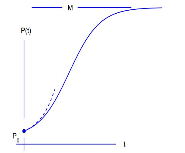
Figure \(\PageIndex{1}\): The graph of a logistic curve \(P(t) = P_{0} M e^{r t} /\left(M-P_{0}+P_{0} e^{r t}\right)\). The dashed curve is the graph of \(p(t)=P_{0} e^{r t}\) showing the close approximation to exponential growth for \(P(t)/M\) small (low density).
Mathematical Model of population growth in a limited environment The growth rate of a population is proportional to the size of the population and to the fraction of the carrying capacity unused by the population.
Example 6.1.2 Examples of computing the derivatives of products and quotients.
- \[\begin{aligned}
P(t)=e^{2 t} \ln t \quad P^{\prime}(t) &=\left[e^{2 t} \ln t\right]^{\prime} \\
&=\left[e^{2 t}\right]^{\prime} \ln t+e^{2 t}[\ln t]^{\prime} \\
&=e^{2 t} 2 \ln t+e^{2 t} \frac{1}{t}
\end{aligned}\] - \[\begin{aligned}
P(t)=\frac{3 t-2}{4+t^{2}} \quad P^{\prime}(t) &=\left[\frac{3 t-2}{4+t^{2}}\right]^{\prime} \\
&=\frac{\left(4+t^{2}\right)[3 t-2]^{\prime}-(3 t-2)\left[4+t^{2}\right]^{\prime}}{\left(4+t^{2}\right)^{2}} \\
&=\frac{\left(4+t^{2}\right) 3-(3 t-2)(0+2 t)}{\left(4+t^{2}\right)^{2}} \\
&=\frac{12-6 t^{2}}{\left(4+t^{2}\right)^{2}}
\end{aligned}\] - \[\begin{aligned}
P(t)=\frac{e^{2 t}}{\ln t} \quad P^{\prime}(t) &=\left[\frac{e^{2 t}}{\ln t}\right]^{\prime} \\
&=\frac{\ln t\left[e^{2 t}\right]^{\prime}-e^{2 t}[\ln t]^{\prime}}{(\ln t)^{2}} \\
&=\frac{(\ln t) e^{2 t} 2-e^{2 t} \frac{1}{t}}{(\ln t)^{2}} \\
&=e^{2 t} \frac{2 t(\ln t)-1}{t(\ln t)^{2}}
\end{aligned}\]
Exercises for Section 6.1, Derivatives of Products and Quotients.
Exercise 6.1.1 The word differentiate means 'find the derivative of'.
Differentiate
- \(P(t)=\frac{e^{-3 t}}{t^{2}}\)
- \(P(t)=e^{2 \ln t}\)
- \(P(t)=e^{t} \ln t\)
- \(P(t)=t^{2} e^{2 t}\)
- \(P(t)=e^{t \ln 2}\)
- \(P(t)=e^{2}\)
- \(P(t)=\left(e^{t}\right)^{5}\)
- \(P(t)=\frac{t-1}{t+1}\)
- \(P(t)=\frac{3 t^{2}-2 t-1}{t^{-} 1}\)
Exercise 6.1.2 Compute \(P^{\prime}\) for:
- \(P(t)=t^{2} e^{t}\)
- \(P(t)=\sqrt{t} e^{\sqrt{t}}\)
- \(P(t)=\frac{t}{1+t^{2}}\)
- \(P(t)=\frac{t+1}{t-1}\)
- \(P(t)=e^{t} \sqrt{1+t}\)
- \(P(t)=t \ln t-t\)
- \(P(t)=t e^{t}-e^{t}\)
- \(P(t)=t^{2} e^{t}-2 t e^{t}+2 e^{t}\)
- \(P(t)=\frac{\sqrt{t}}{\ln t}\)
- \(P(t)=e^{t} \ln t\)
- \(P(t)=\frac{1}{\ln t}\)
- \(P(t)=e^{(t \ln t)}\)
- \(P(t)=10 \frac{e^{0.2 t}}{9+e^{0.2 t}}\)
- \(P(t)=\frac{20}{1+19 e^{-0.1 t}}\)
Exercise 6.1.3 Give reasons for steps (i) − (v) in Equations \ref{6.4} proving Theorem 6.1.1, the derivative of a product formula.
Exercise 6.1.4 Give reasons for steps (i) − (vi) in Equations \ref{6.6} proving Theorem 6.1.2, the derivative of a quotient formula.
Exercise 6.1.5 Write an equation that interprets the mathematical model of logistic growth, Mathematical Model 6.1.1 on page 275, and show that it can be written in the form of Equation \ref{6.9}.
Exercise 6.1.6 Is there an example of two functions, \(u(x)\) and \(v(x)\), for which \([u(x) \times v(x)]^{\prime} = u ^{\prime} (x) \times v ^{\prime} (x)\)?
Exercise 6.1.7 Is there an example of two functions, \(u(x)\) and \(v(x)\), for which \(\left[\frac{u(x)}{v(x)}\right]^{\prime}=\frac{u^{\prime}(x)}{v^{\prime}(x)}\)?
Exercise 6.1.8 An examination of 1000 people showed that 41 were carriers (heterozygotic) of the gene for cystic fibrosis. Let p be the proportion of all people who are carriers of cystic fibrosis. We can not say with certainty that \(p = 41/1000\). For any number \(p\) in \([0,1]\), let \(L(p)\) be the likelihood of the event that 41 of 1000 people are carriers of cystic fibrosis given that the probability of being a carrier is \(p\). Then
\[L(p)=\left(\begin{array}{c}
1000 \\
41
\end{array}\right) p^{41} \times(1-p)^{959}\]
where \(\left(\begin{array}{c}
1000 \\
41
\end{array}\right)\) is a constant1 approximately equal to \(1.3 \times 10^{73} \).
- Compute \(L ^{\prime} (p)\).
- Find the value \(\hat{p}\) of p for which \(L ^{\prime} (p) = 0\) and compute \(L(\hat{p})\).
The value \(L(\hat{p})\) is the maximum value of \(L(p)\) and \(\hat{p}\) is called the maximum likelihood estimator of \(p\).
Exercise 6.1.9 An examination of 1000 people showed that 41 were carriers (heterozygotic) of the gene for cystic fibrosis. In a second, independent examination of 2000 people, 79 were found to be carriers of cystic fibrosis. Let \(p\) be the proportion of all people who are carriers of cystic fibrosis. For any number \(p\) in \([0,1]\), let \(L(p)\) be the likelihood of finding that 41 of 1000 people in one study and 79 out of 2000 people in a second independent study are carriers of cystic fibrosis given that the probability of being a carrier is \(p\). Then
\[L(p)=\left(\begin{array}{c}
1000 \\
41
\end{array}\right) p^{41} \times(1-p)^{959} \times\left(\begin{array}{c}
2000 \\
79
\end{array}\right) p^{79} \times(1-p)^{1921}\]
where \(\left(\begin{array}{c}
1000 \\
41
\end{array}\right) \doteq 1.3 \times 10^{73}\) and \(\left(\begin{array}{c}
2000 \\
79
\end{array}\right) \doteq 1.4 \times 10^{143}\) are constants.
- Simplify \(L(p)\).
- Compute \(L ^{\prime} (p)\).
- Find the value \(\hat{p}\) of \(p\) for which \(L ^{\prime} (p) = 0\).
The value \(L(\hat{p})\) is the maximum value of \(L(p)\) and \(\hat{p}\) is called the maximum likelihood estimator of \(p\).
Exercise 6.1.10 A bird searches bushes in a field for insects. The total weight of insects found after \(t\) minutes of searching a single bush is given by \(w(t)=\frac{2 t}{t+4}\) grams. Draw a graph of w. From your graph, does it appear that a bird should search a single bush for more than 10 minutes? It takes the bird one minute to move from one bush to another. How long should the bird search each bush in order to harvest the most insects in an hour of feeding?
Exercise 6.1.11 Van der Waal’s equation for gasses at high pressure (20 to 1000 atmospheres, say) is
\[\left(P+\frac{n^{2} \times a}{V^{2}}\right)(V-n * b)=n * R * T \label{6.10}\]
where \(n\) and \(R\) are, respectively, the number of moles and the ideal gas law constant, and \(a\) and \(b\) are constants specific to the gas under study.
- Find \(\frac{d P}{d T}\) under the assumption that the volume, \(V\), is constant.
- Find \(\frac{d P}{d T}\) under the assumption that the temperature, \(T\), is constant.
Exercise 6.1.12 Let
\[P(t)=\frac{u(t)}{v(t)}=u(t) \times(v(t))^{-1}\]
Use the product rule and power chain rule to show that
\[P^{\prime}(t)=\frac{u^{\prime}(t) v(t)-u(t) v^{\prime}(t)}{v^{2}(t)}\]
Exercise 6.1.13 Let \(P(t) = u(t) \times v(t)\). Then
\[\ln P(t)=\ln (u(t) \times v(t))=\ln u(t)+\ln v(t) \label{6.11}\]
Compute the derivative of the two sides of Equation \ref{6.11} using the logarithm chain rule and show that
\[P^{\prime}(t)=u(t) v^{\prime}(t)+u^{\prime}(t) v(t)\]
Exercise 6.1.14 Let \(P(t) = u(t)/v(t)\). Then
\[\ln P(t)=\ln \left(\frac{u(t)}{v(t)}\right)=\ln u(t)-\ln v(t) \label{6.12}\]
Compute the derivative of the two sides of Equation \ref{6.12} using the logarithm chain rule and show that
\[P^{\prime}(t)=\frac{u(t) v^{\prime}(t)-u^{\prime}(t) v(t)}{v^{2}(t)}\]
Exercise 6.1.15 A useful special case of the quotient formula is the reciprocal formula: If \(u(t)\) has a derivative and \(u(t) \neq 0\) and
\[P(t)=\frac{1}{u(t)}\]
then
\[P^{\prime}(t)=\frac{-1}{u^{2}(t)} u^{\prime}(t)\]
Prove the formula using logarithmic differentiation. That is, write
\[\ln P(t)=\ln \left(\frac{1}{u(t)}\right)=-\ln u(t)\]
and compute the derivatives of both sides using the logarithm chain rule. We write the formula as
\[\left[\frac{1}{u(t)}\right]^{\prime}=\frac{-1}{u^{2}(t)} u^{\prime}(t) \quad \text{Reciprocal Rule} \label{6.13}\]
Exercise 6.1.16 Use Equations \ref{6.2} and \ref{6.13} to compute the derivative of
\[P(t)=\frac{t^{2}-1}{t^{2}+1}=\left(t^{2}-1\right) \frac{1}{t^{2}+1}\]
Exercise 6.1.17 Provide reasons for steps (ii), (iii), and (iv) in Equations 6.8 computing the derivative of the logistic function. Step (vii) is a hassle. One has to first compute \(1 − P(t)/M\) where \(P(t)=P_{0} M e^{k t} /\left(M-P_{0}+P_{0} e^{k t}\right)\). Give it a try.
Exercise 6.1.18 Sketch the graphs of the logistic curve
P(t)=\frac{P_{0} M e^{r t}}{M-P_{0}+P_{0} e^{r t}}
for
- \(r=0.5 \quad M=20 \quad P_{0}=1, \quad 15, \quad 20, \quad \text{and} \quad 30 \quad 0 \leq t \leq 20\)
- \(r=0.1 \quad M=20 \quad P_{0}=1, \quad 15, \quad 20, \quad \text{and} \quad 30 \quad 0 \leq t \leq 70\)
- \(P_{0}=1 \quad M=20 \quad r=0.1, \quad 0.3, \quad 0.5, \text{and} 0.7 \quad 0 \leq t \leq 50\)
- \(P_{0}=1 \quad r=0.2 \quad M=10, \quad 15, \quad 20, \quad \text{and} 25 \quad 0 \leq t \leq 50\)
Exercise 6.1.19 For what population size is the growth rate \(P^{\prime}\) of the logistic population function the greatest? The equation
\[P^{\prime}(t)=r P(t)\left(1-\frac{P(t)}{M}\right)\]
provides an answer. Observe that \(y=r p(1-p / M)=r p-(r / M) p^{2}\) is a quadratic whose graph is a parabola.
The answer to this question is important, for the population size for which \(P^{\prime}\) is greatest is that population that wildlife managers may wish to maintain to provide maximum growth.
Exercise 6.1.20 Crows on the west coast of Canada feed on a mollusk called a whelk (shown in Figure \(\PageIndex{2}\))2. The crows break the whelk shell to obtain the meat inside by lifting the whelk to a height of about 5 meters and dropping it onto a rock.
Copyright permission to use the figures from Reto Zach’s papers was given by Brill Publishers, PO Box 9000, 2300 PA Leiden, The Netherlands.
Reto Zach (1978,1979) investigated the behavior of crow feeding as an example of decision making while foraging for food, and concluded that crows break the whelk in a manner that minimized their effort (optimal foraging). Crows find whelks in the intertidal zone near the water, carry it towards the land, fly vertically and drop it from a height for breaking. The vertical ascent and drop are repeated until the whelk breaks. Zach made two interesting observations:
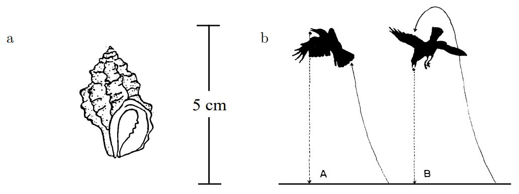
Figure \(\PageIndex{2}\): a. Schematic drawing of a whelk (Zach, 1978, Figure 1). b. “Flights during dropping. Some crows release whelk at highest point of flight and are unable to see whelk fall (A). Most crows lose some height before dropping but are able to see whelk fall (B).” ( ibid., Fig 6.)
- The crows fed only on large whelk. When large whelk were not available, crows selected another food source.
- Consistently the crows dropped the whelk from a height of about 5 meters.
Zach gathered whelks from the intertidal zone, separated them into small, medium, and large categories, and dropped them repeatedly at a given height until they broke. He repeated this at varying heights, and his results are shown in Figure \(\PageIndex{3}\).
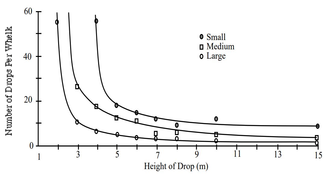
Figure \(\PageIndex{3}\): Mean number of drops required for breaking large, medium and small whelks dropped from various heights. Curves fitted by eye. (Zach, 1979, Figure 2.)
We read data from the graph for \(N\) the number of drops required to break a medium sized whelk from a height \(H\) and find that the following hyperbola matches the data:
\[N=1+\frac{1}{-0.103+0.0389 H} \quad H \geq 2 \label{6.14}\]
Zach reasoned that the work, \(W\), done to break a whelk by dropping it \(N\) times from a height \(H\) was equal to \(N \times H\). For a medium sized whelk,
\[W=N \times H=\left(1+\frac{1}{-0.103+0.0389 H}\right) \times H \quad H \geq 2 \label{6.15}\]
- Graph Equation \ref{6.15}. From your graph, find (approximately) the value of \(H\) for which \(W\) is a minimum.
- Compute \(\frac{d W}{d H}\) from Equation \ref{6.15}. Find the value \(H_0\) of \(H\) for which \(\frac{dW}{dH} = 0\) and the value \(W_0\) of \(W\) corresponding \(H_0\).
- Explain why the answers to the two previous parts are equal (or very close).
- Interpret the quotient \(W_{0}/H_{0}\).
- Data for large whelk (read from an enlargement of Figure \(\PageIndex{3}\)) are shown in Table 6.1. From the graph in Figure \(\PageIndex{3}\), read the number of drops required to break a large whelk for Height= 2m and Height= 3m and complete the table.
| Height of Drop | Number of Drops | \([\text{Number of Drops } - 1]^{-1}\) |
|---|---|---|
| 2 | 0.019 | |
| 3 | ||
| 4 | 6.7 | 0.18 |
| 5 | 4.8 | |
| 6 | 3.8 | 0.36 |
| 7 | 3.2 | 0.45 |
| 8 | 2.5 | 0.67 |
| 10 | 2.6 | 0.63 |
| 15 | 1.9 | 1.1 |
- Find an equation of a hyperbola that matches the data for a large whelk. Note: The number of drops is clearly at least 1, use the equation \[N=1+\frac{1}{a+b H}\] and find \(a\) and \(b\) to match the data. The previous equation can be changed to \[N-1=\frac{1}{a+b H}, \quad \frac{1}{N-1}=a+b H\] Therefore a graph of \(\frac{1}{N-1}\) versus H should be approximately linear, and the coefficients of line fit to that data will be good values for \(a\) and \(b\). Find \(a\) and \(b\).
- Find the value of \(H_0\) of \(H\) that minimizes the work required to break a large whelk.
- Find the minimum amount of work required to break a large whelk. On average, how many drops does it take to break a large whelk from the optimum height, \(H_0\)?
Summary. The work required to break a medium sized whelk is twice that require to break a large whelk, and the optimum height from which to drop a large whelk is 6.1 meters, reasonably close to the 5.58 meters obtained by Zach.
A similar behavior is observed in sea gulls feeding on mussels. A large mussel broken on the second drop by a gull is shown in Figure \(\PageIndex{4}\); attached to the large mussel shell is a small mussel that the gull did not bother to break.
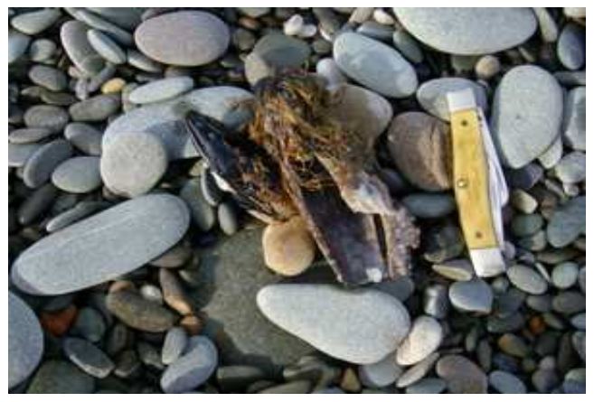
Figure \(\PageIndex{4}\): A large mussel shell broken by a gull on the second drop. Attached to it is a small mussel that the gull did not break. (Photo by JLC)
1 \(\left(\begin{array}{l}
n \\
r
\end{array}\right)\) is the number of \(r\) member subsets of a set with \(n\) elements, and is equal to \(\frac{n !}{r !(n-r) !}\).
2 Reto Zach, Selection and dropping of whelks by northwestern crows, Behaviour 67 (1978), 134-147. Reto Zach, Shell dropping: Decision-making and optimal foraging in northwestern crows, Behaviour 68 (1979), 106-117.