6.2: The chain rule

The Power Chain Rule, the Exponential Chain Rule, and the Logarithm Chain Rule have a common pattern and we list all three to show the similarity:

If a function, \(u(t)\), has derivative then

\[\begin{aligned}
\left[u(t)^{n}\right]^{\prime}=n u(t)^{n-1} \times[u(t)]^{\prime} \quad &\text{Power Chain Rule}\\ \left[e^{u(t)}\right]^{\prime}=n e^{u(t)} \times[u(t)]^{\prime} \quad &\text{Exponential Chain Rule}\\
[\ln u(t)]^{\prime}=\frac{1}{u(t)} \times[u(t)]^{\prime} \quad &\text{Logarithm Chain Rule}\\
\end{aligned}\]

All three of these are of the form

Note

\[[G(u(t))]^{\prime}=G^{\prime}(u(t)) \times[u(t)]^{\prime} \quad \textbf{ Chain Rule } \label{6.16}\]

where

\[G^{\prime}(u(t)) \text { means } G^{\prime}(u), \text { the derivative of } G \text { with respect to } u \text {. }\]

Consider

\[\begin{array}\
&G(u) & G^{\prime}(u) & G(u(t)) & G^{\prime}(u(t)) \times[u(t)]^{\prime} & \text { Chain Rule }\\
&u^{n} & n u^{n-1} & (u(t))^{n} & n u(t)^{n-1} \times[u(t)]^{\prime} & \text { Power }\\
&e^{u} & e^{u} & e^{u(t)} & e^{u(t)} \times[u(t)]^{\prime} & \text { Exponential }\\
&\ln u & \frac{1}{u} & \ln (u(t)) & \frac{1}{u(t)} \times[u(t)]^{\prime} & \text { Logarithm }\\
\end{array}\]

\(G ^{\prime} (u)\) in the second column is the derivative with respect to \(u\), the independent variable of \(G\), and will often be computed using a Primary Formula.

Example 6.2.1 Compute \(F ^{\prime} (t)\) for \(F(t)=\left(1-t^{2}\right)^{3}\). Let

\[\begin{gathered}
G(z)=z^{3} \quad \text { and } u(t)=1-t^{2} . \text { Then } F(t)=G(u(t)) \\
G^{\prime}(z)=3 z^{2} \quad \text { and } \quad[u(t)]^{\prime}=-2 t \\
G^{\prime}(u(t))=3(u(t))^{2}=3\left(1-t^{2}\right)^{2}
\end{gathered}\]

and

\[F^{\prime}(t)=G^{\prime}(u(t))[u(t)]^{\prime}=3\left(1-t^{2}\right)^{2}(-2 t)\]

In the form \(G(u(t))\), \(G(u)\) may be called the 'outside' function and \(u(t)\) may be called the inside function. Consider

\[\begin{array}\
&\text { For } & \text{ Outside } & \text { Inside }\\
&\sqrt{1+t^{2}} & G(u)=\sqrt{u} & u(t)=1+t^{2}\\
&\frac{1}{1+e^{t}} & G(u)=\frac{1}{u} & u(t)=1+e^{t}\\
&e^{-t^{2} / 2} & G(u)=e^{u} & u(t)=-t^{2} / 2\\
&\ln \left(e^{t}+1\right) & G(u)=\ln u & u(t)=e^{t}+1\\
\end{array}\]

Theorem 6.2.1

Chain Rule. Suppose \(G\) and u are functions that have derivatives and \(G( u(t) )\) is defined for all numbers \(t\). Then \(G( u(t) )\) has a derivative for all \(t\) and

\[[G(u(t))]^{\prime}=G^{\prime}(u(t)) \times[u(t)]^{\prime} \label{6.17}\]

Proof: The argument is similar to that for the exponential chain rule. The difference is that we now have a general function \(G(u)\) rather than the specific functions \(e ^u \). We argue only for \(u\) an increasing function, and we need Theorem 4.2.1, The Derivative Requires Continuity.

Let \(F=G \circ u\) (\(F(t)=G(u(t))\) for all \(t\))

\[\begin{aligned}
F^{\prime}(a) &=\lim _{b \rightarrow a} \frac{F(b)-F(a)}{b-a} \\
&=\lim _{b \rightarrow a} \frac{G(u(b))-G(u(a))}{b-a} \\
&=\lim _{b \rightarrow a} \frac{G(u(b))-G(u(a))}{u(b)-u(a)} \lim _{b \rightarrow a} \frac{u(b)-u(a)}{b-a} \quad u(b)-u(a) \neq 0 \\
&=G^{\prime}(u(a)) u^{\prime}(a)
\end{aligned}\]

The conclusion that

\[\lim _{b \rightarrow a} \frac{G(u(b))-G(u(a))}{u(b)-u(a)}=G^{\prime}(u(a))\]

requires some support.

\[\text{In Figure } \PageIndex{5}, \text{ the slope of the secant is } \quad \frac{G(u(b))-G(u(a))}{u(b)-u(a)}.\]

Because \(u ^{\prime} (a)\) exists, \(u(b) \rightarrow u(a)\) as \(b \rightarrow a\). The slope of the secant approaches the slope of the tangent as \(u(b) \rightarrow u(a)\), and

\[\lim _{b \rightarrow a} \frac{G(u(b))-G(u(a))}{u(b)-u(a)}=G^{\prime}(u(a))\]

End of Proof.

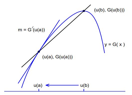
Figure \(\PageIndex{5}\): Graph of a function \(y=G(x)\). As \(b \rightarrow a\), \((G( u(b) ) − G( u(a) ))/(u(b) − u(a)) \rightarrow G ^{\prime} ( u(a) )\).

Example 6.2.2 Repeated use of the chain rule allows computation of derivatives of some quite complex functions.

Problem. Compute the derivative of

\[F(t)=e^{\sqrt{\ln t}} \quad t>1 \quad \text { so that } \quad \ln t>0.\]

Solution. We peel the layers off from the outside. \(F(t)\) can be thought of as

\[F(t)=G(H(K(t))), \quad \text { where } \quad G(z)=e^{z}, \quad H(x)=\sqrt{x}, \quad \text { and } \quad K(t)=\ln t\]

\[\begin{aligned}
{\left[e^{\sqrt{\ln t}}\right]^{\prime} } &=e^{\sqrt{\ln t}}[\sqrt{\ln t}]^{\prime} & G(z)=e^{z}, & G^{\prime}(z)=e^{z} \\
&=e^{\sqrt{\ln t}} \frac{1}{2 \sqrt{\ln t}}[\ln t]^{\prime} & H(x)=\sqrt{x}, & H^{\prime}(x)=\frac{1}{2 \sqrt{x}} \\
&=e^{\sqrt{\ln t}} \frac{1}{2 \sqrt{\ln t}} \frac{1}{t} & K(t)=\ln t, & K^{\prime}(t)=\frac{1}{\mathrm{t}}
\end{aligned}\]

Extreme Problem. Argh! Compute the derivative of

\[F(t)=\left(1+\sqrt{\ln \frac{1-t}{1+t}}\right)^{4}\]

\[\begin{aligned}
&\left[\left(1+\sqrt{\ln \frac{1-t}{1+t}}\right)^{4}\right]^{\prime}=4\left(1+\sqrt{\ln \frac{1-t}{1+t}}\right)^{3}\left[1+\sqrt{\ln \frac{1-t}{1+t}}\right]^{\prime}\\
&=4\left(1+\sqrt{\ln \frac{1-t}{1+t}}\right)^{3}\left(0+\frac{1}{2} \frac{1}{\sqrt{\ln \frac{1-t}{1+t}}}\left[\ln \frac{1-t}{1+t}\right]^{\prime}\right)\\
&=4\left(1+\sqrt{\ln \frac{1-t}{1+t}}\right)^{3} \frac{1}{2} \frac{1}{\sqrt{\ln \frac{1-t}{1+t}}}\left(\frac{1}{\frac{1-t}{1+t}}\left[\frac{1-t}{1+t}\right]^{\prime}\right)\\
&=4\left(1+\sqrt{\ln \frac{1-t}{1+t}}\right)^{3} \frac{1}{2} \frac{1}{\sqrt{\ln \frac{1-t}{1+t}}} \frac{1}{1-t} \frac{(1+t)(-1)-(1-t) 1}{(1+t)^{2}}
\end{aligned}\]

The chain rule is an investment in the future. It does not immediately expand the collection of functions for which we can compute the derivative. To use the chain rule on \(G( u(t) )\) we need \(G ^{\prime} (u)\) which requires a Primary derivative formula. The relevant Primary derivative formulas so far developed are the power, exponential and logarithm Primary formulas, for which we have already developed chain rules. In the next chapter, we develop the Primary formula

\[[\sin t]^{\prime}=\cos t\]

Then from the chain rule of this section, we immediately have the chain rule

\[[\sin (u(t))]^{\prime}=\cos (u(t)) u^{\prime}(t)\]

Using this we can, for example, compute \([\sin (\pi t)]^{\prime}\) as

\[\begin{aligned}
{[\sin (\pi t)]^{\prime} } &=\cos (\pi t)[\pi t]^{\prime} \\
&=\cos (\pi t) \pi
\end{aligned}\]

Leibnitz notation. The Leibnitz notation makes the chain rule look deceptively simple. For \(G(u(t))\) one has

\[[G(u(t))]^{\prime}=\frac{d G}{d t} \quad G^{\prime}(u(t))=\frac{d G}{d u} \quad[u(t)]^{\prime}=\frac{d u}{d t}\]

Then the chain rule is

\[\frac{d G}{d t}=\frac{d G}{d u} \frac{d u}{d t}\]

Example 6.2.3 Find \(\frac{dy}{dt}\) for \(y(t)=\left(1+t^{4}\right)^{7}\). \(y(t)\) is the composition of \(G(u) = u ^7\) and \(u(t) = 1 + t ^4 \). Then

\[\begin{aligned}
&\frac{d G}{d u}=\frac{d}{d u} u^{7} \quad=7 u^{6}\\
&\frac{d u}{d t}=\frac{d}{d t}\left(1+t^{4}\right)=4 t^{3}\\
&\frac{d G}{d t}=\frac{d G}{d u} \frac{d u}{d t} \quad=7 u^{6} \times 4 t^{3}=7\left(1+t^{4}\right)^{6} 4 t^{3}
\end{aligned}\]

 

Exercises for Section 6.2, The chain rule.

Exercise 6.2.1 Use the chain rule to differentiate \(P(t)\) for

1. \(P(t)=e^{\left(-t^{2}\right)}\)
2. \(P(t)=\left(e^{t}\right)^{2}\)
3. \(P(t)=e^{2 \ln t}\)
4. \(P(t)=\ln e^{2 t}\)
5. \(P(t)=\ln (2 \sqrt{t})\)
6. \(P(t)=\sqrt{2 \ln t}\)
7. \(P(t)=\sqrt{e^{2 t}}\)
8. \(P(t)=\sqrt{e^{\left(-t^{2}\right)}}\)
9. \(P(t)=\left(t+e^{-2 t}\right)^{4}\)
10. \(P(t)=\left(1+e^{\left(-t^{2}\right)}\right)^{-1}\)
11. \(P(t)=\frac{3}{4}\left(1-x^{2} / 16\right)^{1 / 2}\)
12. \(P(t)=(t+\ln (1+2 t))^{2}\)

Exercise 6.2.2 Use the Leibnitz notation for the chain rule to find \(\frac{dy}{dt}\) for

1. \(y(t)=e^{\left(-t^{2}\right)}\)
2. \(y(t)=\left(e^{t}\right)^{2}\)
3. \(y(t)=e^{2 \ln t}\)
4. \(y(t)=\left(\frac{e^{t}}{1+e^{t}}\right)^{2}\)
5. \(y(t)=\sqrt{2 t^{2}-t+1}\)
6. \(y(t)=\left(t^{2}+1\right)^{3}\)

Compare your answers for a - c with those of Exercise 6.2.1 a - c.

Exercise 6.2.3 In Chapter 7 we show that \([\cos (t)]^{\prime}=-\sin (t)\). Use this formula and \([\sin t]^{\prime}=\cos t\) written earlier in this chapter to differentiate:

1. \(y(t)=\cos (2 t)\)
2. \(y(t)=\sin \left(\frac{\pi}{2} t\right)\)
3. \(y(t)=e^{\cos t}\)
4. \(y(t)=\cos \left(e^{t}\right)\)
5. \(y(t)=\sin (\cos t)\)
6. \(y(t)=\sin \left(\cos e^{t}\right)\)
7. \(y(t)=\ln (\sin t)\)
8. \(y(t)=\sec t=(\cos t)^{-1}\)
9. \(y(t)=\ln \left(\cos \left(e^{t}\right)\right)\)
10. \(y(t)=\ln \left(\cos \left(e^{\sin t}\right)\right)\)

Exercise 6.2.4 The Doppler effect. You are standing 100 meters south of a straight train track on which a train is traveling from west to east at the speed 30 meters per second. See Figure 6.2.4. Let \(y(t)\) be the distance from the train to you and \(|x(t)|\) be the distance from the train to the point on the track nearest you; \(x(t)\) is negative when the train is west of the point on the track nearest you.

1. Write \(y(t)\) in terms of \(x(t)\).
2. Find \(y ^{\prime} (t)\) for a time t at which \(x(t) = −200\)
3. Time is measured so that \(x(0) = 0\). Write an equation for \(x(t)\).
4. Write an equation for \(y ^{\prime} (t)\) in terms of \(t\).
5. The whistle from the train projects sound waves at frequency \(f\) cycles per second. The frequency, \(f_L\), of the sound reaching your ear is \[f_{L}(t)=\frac{331.4}{331.4+y^{\prime}(t)} f \frac{\text { cycles }}{\text { second }} \label{6.18}\] 331.4 m/s is the speed of sound in air. Draw a graph of \(f_{L}(t)\) assuming \(f = 500\).

Derivation of Equation \ref{6.18} for the Doppler effect. A sound of frequency \(f\) traveling in still air has wave length (331.4 m/s)/(f cycles/s) = (331.4/f) m/cycle. If the source of the sound is moving at a velocity v with respect to a listener, the wave length of the sound reaching the listener is \((331.4 \mathrm{~m} / \mathrm{s}) /(f \text { cycles } / \mathrm{s})=(331.4 / \mathrm{f}) \mathrm{m} / \text { cycle. }\) These waves travel at 331.4 m/sec, and the frequency \(f_L\) of these waves reaching the listener is

\[f_{L}=\frac{331.4 \mathrm{~m} / \mathrm{s}}{((331.4+v) / f) \mathrm{m} / \mathrm{cycle}}=\frac{331.4}{331.4+v} f \frac{\text { cycles }}{\text { second }}\]

High frequency sound waves may be used to measure the rate of blood flow in an artery. A high frequency sound is introduced on the skin surface above the artery, and the frequency of the waves reflected from the arterial flow is measured. The difference in frequencies emitted and received is used to measure blood velocity.

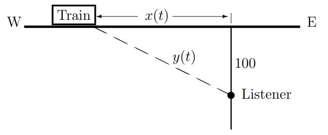
Figure for Exercise 6.2.4 A train and track with listener location. As drawn, \(x(t)\) is negative

Exercise 6.2.5 Air is being pumped into a spherical balloon at the rate of \(1000 \mathrm{~cm}^{3} / \mathrm{min}\). At what rate is the radius of the balloon increasing when the volume is \(3000 \mathrm{~cm}^{3}\)? Note: \(V(t)=\frac{4}{3} \pi r^{3}(t)\).

Exercise 6.2.6 Consider a spherical ice ball that is melting. A reasonable model is:

Mathematical Model.

1. The rate at which heat is transferred to the ice ball is proportional to the surface area of the ice ball.
2. The rate at which the ball melts is proportional to the rate at which heat is transferred to the ball.

The volume, \(V\), of a sphere of radius \(r\) is \(\frac{4}{3} \pi r^{3}\) and its surface area, \(S\), is \(4 \pi r ^{2} \). From 1 and 2 we conclude that the rate of change of volume of the ice ball is proportional to the surface area of the ice ball.

1. Write an equation representative of the previous italicized statement.
2. As the ball melts, \(V\), \(r\), and \(S\) change with time. Differentiate \(V(t)=\frac{4}{3} \pi r^{3}(t)\) to obtain \[V^{\prime}(t)=4 \pi r^{2}(t) r^{\prime}(t)\]
3. Use your equation from (a) and the equation from (b) to show that \[r^{\prime}(t)=K \quad \text { where } K \text { is a constant }\]
4. Why should \(K\) be negative?
5. Because \(K\) should be negative, we write \[r^{\prime}(t)=-K\] A good candidate for \(r(t)\) is \[r(t)=-K t+C \quad \text{ where } C \text{ is a constant}\] Why?
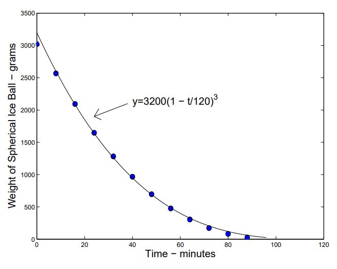
6. Only discussion included in this part. With \(r(t)=-K T+C\) we find that \[W(t)=A(1-t / B)^{3} \quad \text { where } W(t) \text { is the weight of the ball }\] and \(A\) and \(B\) are constants. In order to test this conclusion, we filled a plastic ball about the size of a volley ball with water and froze it to \(-14 ^{\circ} C\) (Figure 6.2.6). One end of a chord (knotted) was frozen into the center of the ball and the other end extended outside the ball as a handle. We removed the plastic and placed the ball in a \(10 ^{\circ} C\) water bath, held below the surface by a weight attached to the ball. At four minute intervals we removed the ball and weighed it and returned it to the bath. The data from one of these experiments is shown in Table 6.2.6 and a plot of the data and of a cubic, \(y=3200(1-t / 120)^{3}\), is shown in the figure of Table 6.2.6. The cubic looks like a pretty good fit to the data, and we might argue that the data is consistent with our model. There are some flaws with the fit of the cubic, however. The cubic departs from the data at both ends. \(y(0) = 3200\), but the ball only weighed 3020 g; the cubic is also above the data at the right end.
7. We found that we could fit the data more closely with an equation of the form \[W(t)=A(1-t / 100)^{\alpha}\] where \(\alpha\) is closer to 2 than to 3. Find values for \(A\) and \(\alpha\). Note: \(\ln W(t)=\ln A+\alpha \ln (1-t / 100)\). Then reasonable estimates of \(\ln A\) and \(\alpha\) are the coefficients of a line fit to the graph of \(\ln w(t)\) versus \(\ln (1 - t/100)\).
8. If the data is not consistent with the model, in what way might the model be deficient?

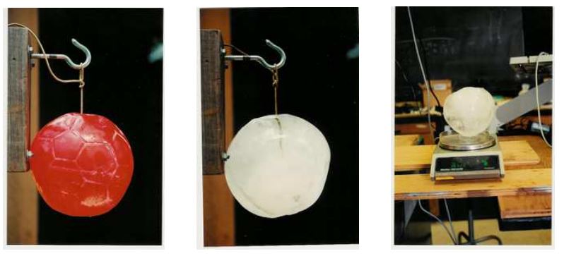
Figure for Exercise 6.2.6 (h) Pictures of an ice ball used in the experiments described in Exercise 6.2.6.

Table for Exercise 6.2.6 Data from an ice ball melt experiment described in Exercise 6.2.6.

Time (m)	Weight (g)
0	3020
4	2567
8	2093
12	1647
16	1282
20	967
24	696
28	476
32	305
36	172
40	82
44	25